SMS Matching and Theory Predictions
After the decomposition of the input model into a sum of SMS, the next steps consist of matching the SMS from the decomposition to the topologies constrained in the database, and computing the relevant signal cross sections (or theory predictions) for comparison with the experimental limits. Fig. 19 schematically shows these two steps.
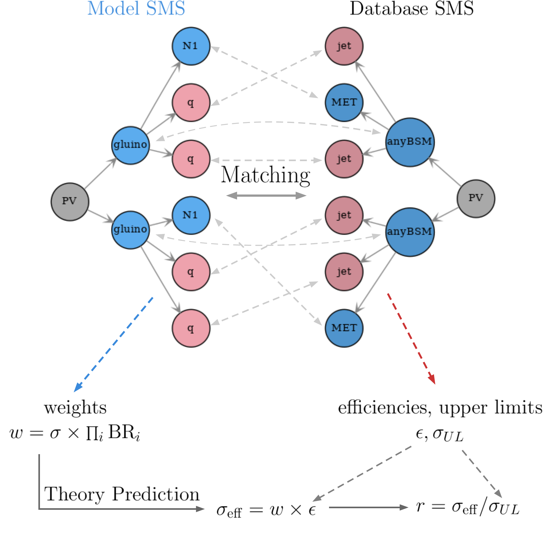
Figure 19: Schematic representation of the matching between SMS topologies generated by the decomposition (Model SMS) and the topologies found in the database (Database SMS), as well as the calculation of the relevant theory predictions and the comparison against the experimental data.
Below we describe in detail the procedure for matching the SMS topologies and for computing the theory predictions.
Matching SMS Topologies
Once the SMS topologies (here called model SMS) representing the input BSM model are created by the decomposition, they have to be matched to the topologies constrained by the Database (database topologies). Two topologies will match if they have the same structure and the corresponding particles appearing in each topology have matching properties (electric charge, color representation, spin,…).1
In the graph language, two SMS match if their the root nodes (primary vertices) match. Any two nodes will be considered matched if:
their canonical names are equal,
their particle attributes match and
their daughter nodes match irrespective of their ordering
With these criteria, the SMS topologies are traversed following a depth-first search until all nodes have been matched (if possible). In order to illustrate this procedure it is useful to consider the example of the model and database topologies shown in Fig. 20.
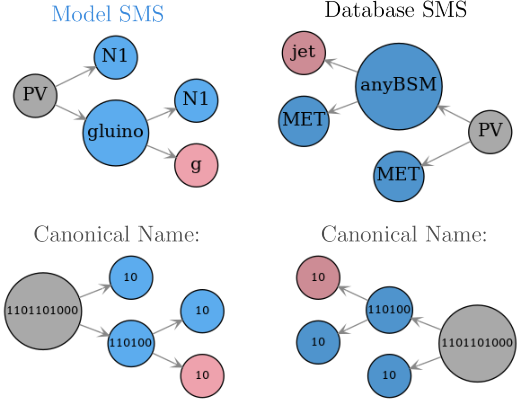
Figure 20: Example of two topologies to be matched and the respective canonical names for their nodes.
The procedure compares the root nodes, which in this example have the same canonical names (this enforces that both SMS have the same structure) and the same particle properties (which is always assumed as true to root nodes). This is indicated by Step 0 in Fig. 21. Hence criteria 1. and 2. for matching two nodes are satisfied.
The next step consists in comparing the root nodes daughters irrespective of their order. In this example these are (gluino, N1) from the model topology and (MET,anyBSM) from the database topology, as shown by. Once again we compare their canonical names and particle properties (Step 1 in Fig. 21). Note that although the particle properties of N1 and anyBSM match, their canonical names are different, hence we only have the following partial matches:
gluino \(\leftrightarrow\) anyBSM
N1 \(\leftrightarrow\) MET
In order to fully match the gluino and anyBSM nodes their daughters must also be compared (Step 2). Since their daughters (g,N1) and (MET,jet) are final state nodes (undecayed) the comparison procedure stops at this level and results in the following matches:
g \(\leftrightarrow\) jet
N1 \(\leftrightarrow\) MET
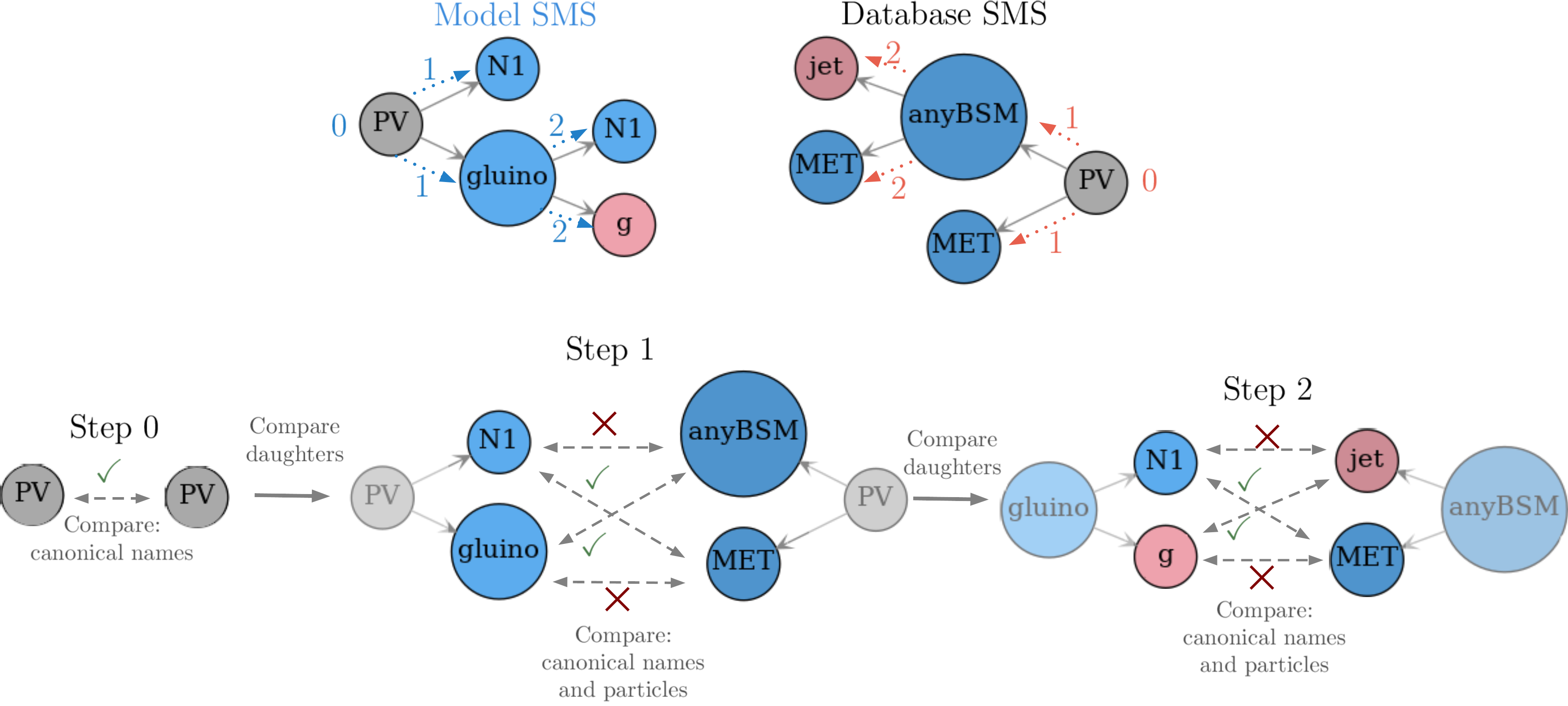
Figure 21: Illustration of the procedure of matching, step by step.
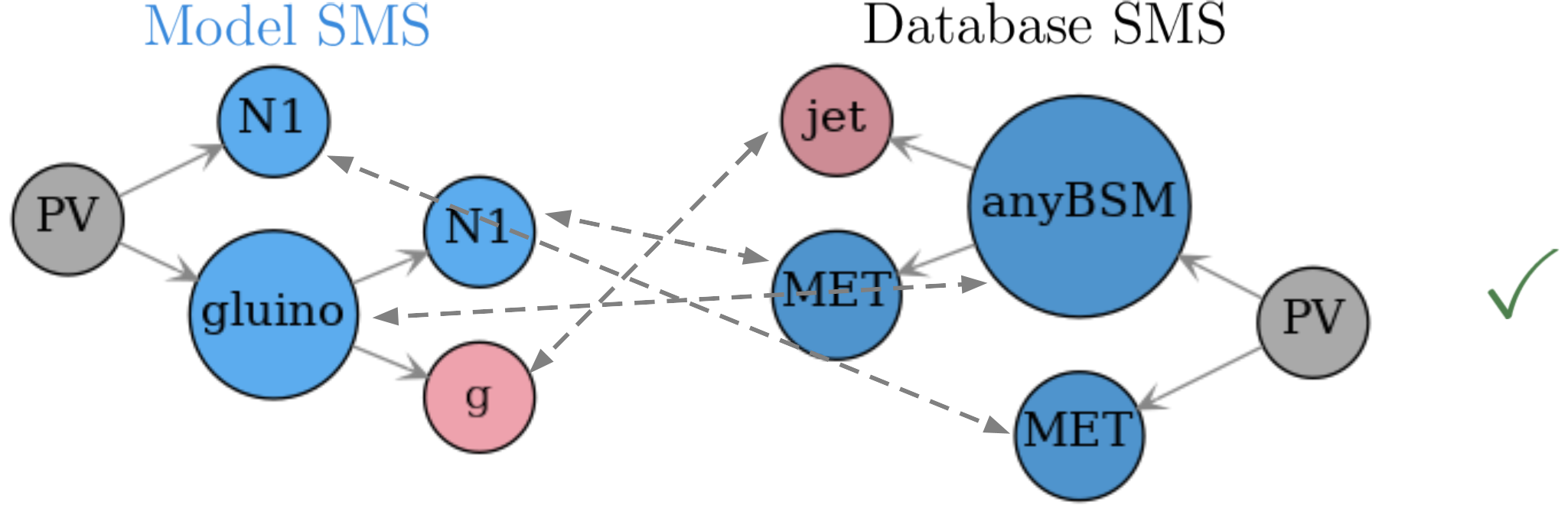
This result finally means a full match for the (gluino,N1) and (anyBSM,MET) pairs, which then means that the root nodes fully match. Consequently the model and database topologies match (see Fig. 22). The procedure just described can be applied to any pair of SMS topologies2 and can also be applied to inclusive topologies with small modifications.
Computing Theory Predictions
Once the SMS topologies coming out of the decomposition have been matched to the database topologies, the relevant (effective) cross-sections need to be computed and compared to the data from a given experimental result (see Fig. 19). As discussed in database, SModelS uses two types of experimental results: UL-type results and EM-type results. Each of them requires slightly different theoretical predictions to be compared against the experimental data.
Theory Predictions for Efficiency Map Results
EM-type results constrain the number of signal events (\(N_s^{\rm SR}\)) in a given signal region (DataSet). Equivalently SModelS considers the limit on the effective cross section \(\sigma_{\rm eff}^{\rm SR} = N_s^{\rm SR}/\mathcal{L}\), where \(\mathcal{L}\) is the search luminosity. In this case the theory prediction to be computed corresponds to the effective cross section given the decomposition output. Note that a single EM-type result usually contains several signal regions (DataSets) and there will be a set of efficiencies (or efficiency maps) for each data set. As a result, several theory predictions (one for each data set) need to be computed.
After the model topologies obtained by the decomposition have been matched to the database topologies, the effective cross section is simply given by the sum over the effective cross sections for each SMS, which corresponds to their weights multiplied by the corresponding efficiencies (see Fig. 23).
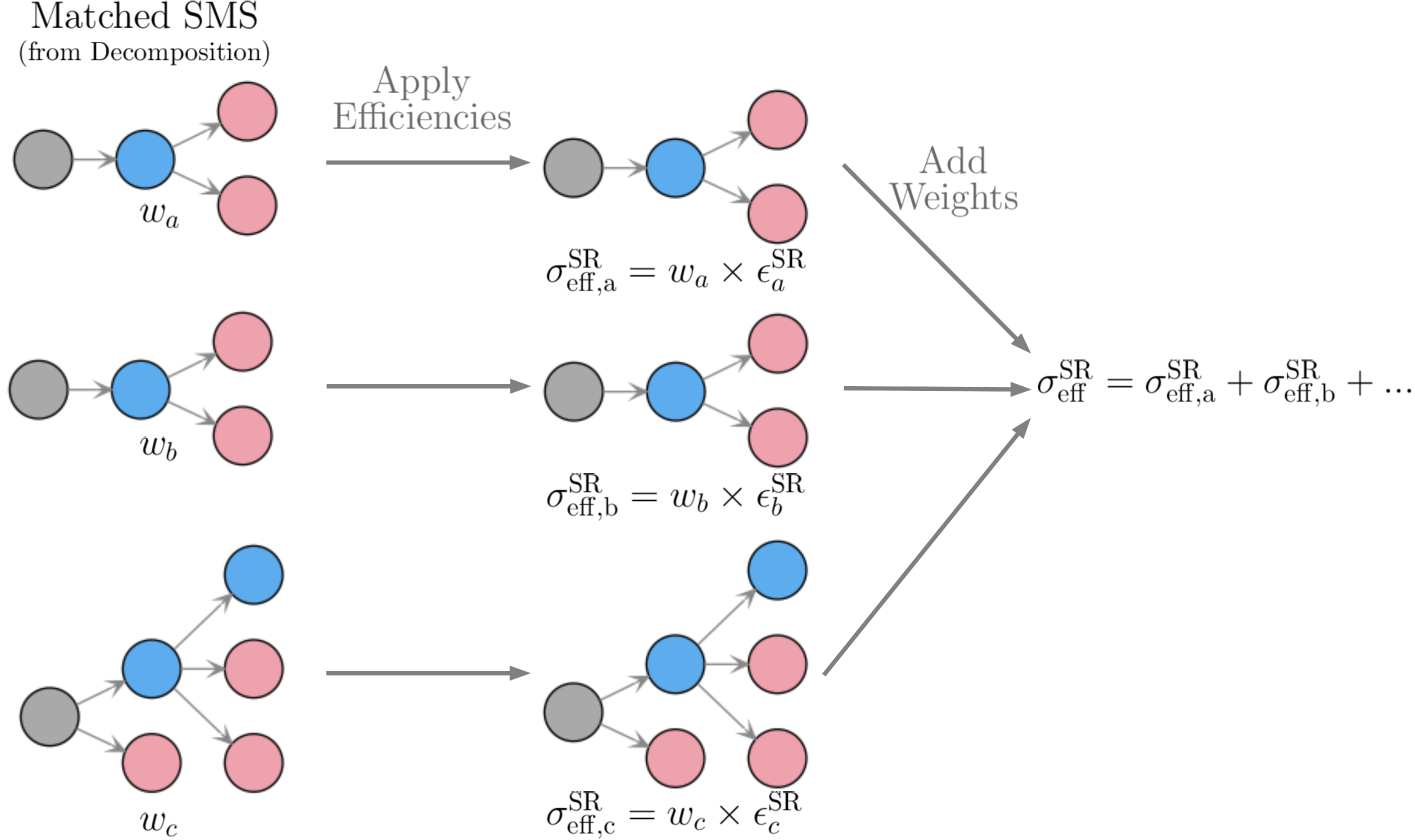
Figure 23: Schematic representation of how the theory prediction value (effective cross section) is computed for the case of EM-type results.
Note that the efficiencies are computed using the efficiency maps for the corresponding DataSet. Finally, \(\sigma_{\rm eff}^{\rm SR}\) can be compared to the signal upper limit for the respective signal region (DataSet). Therefore it is convenient to define:
where \(\sigma_{\rm eff,UL}^{\rm SR} = N_{s,{\rm UL}}^{\rm SR}/\mathcal{L}\) is the 95% C.L. upper limit on the effective cross section. Hence, values of \(r\) larger than one can mean the input model violates the 95% C.L. limit set by the corresponding EM-type result.
For EM-type results where a covariance matrix or statistical model is available, it is possible to combine all the signal regions (see Combination of Signal Regions). In this case the final theory prediction corresponds to the sum of effective cross sections over all signal regions (\(\sum_{\rm SR} \sigma_{\rm eff}^{\rm SR}\)) and the upper limit is computed for this sum.
Theory Predictions for Upper Limit Results
UL-type results constrains the weight (\(\sigma \times BR\)) of a given SMS. Therefore the theory prediction in this case simply corresponds to the weight of the matched topologies. However, a few details have to be taken into account when comparing the weights to the corresponding upper limits.
First, a given UL-type result constraint can be inclusive over final states (i.e. both electrons and muons may be allowed as final states). In this case the weights of all matched SMS corresponding to these final states must be included. However, the selected SMS may differ in their BSM properties (such as masses and/or widths) and the experimental limit (see Upper Limit constraint) assumes that all the topologies appearing in the constraint have the same efficiency, which typically implies that the distinct topologies have the same mass arrays and widths. As a result, the selected SMS must be grouped into clusters of similar efficiencies. In the simplest case, where the upper limit result corresponds to a single signal region, one could assume that the SMS efficiency is inversely proportional to its upper limit: \(\epsilon_a \sim 1/\sigma_{UL,a}\). Hence SMS with similar upper limits have similar efficiencies and can be clustered together, as illustrated in Fig. 24. Mode details about the clustering procedure can be found in Clustering Topologies.
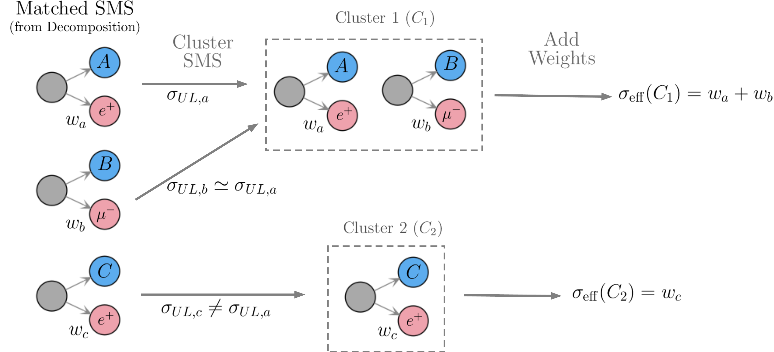
Figure 24: Example of how the theory prediction values (effective cross sections) are computed for the case of UL-type results.
Once the matched SMS have been grouped into cluster the effective cross section can finally computed as the sum of the weights over the topologies within each cluster (see Fig. 24). In this case the following \(r\)-value is defined:
where \(\sigma_{\rm UL}\) is the 95% C.L. upper limit on the effective cross section obtained from the upper limit maps and the sum is over all SMS belonging to the same cluster. Hence, values of \(r\) larger than one can mean the input model violates the 95% C.L. limit set by the corresponding UL-type result.
Theory predictions are computed using the theoryPredictionsFor method
Clustering Topologies
As discussed in Theory Predictions for UL, in order to cluster the topologies it is necessary to determine whether two SMS are similar for a given Experimental Result, which usually means similar efficiencies. Although the efficiencies are related to the cross section upper limits (\(\sigma_{\rm UL}\)), the assumption that they are inversely proportional to the efficiencies is only valid for searches with a single signal region, which is rarely the case. However, if two SMS have similar properties (i.e. BSM masses and widths) and their upper limits are nearly equal, it is reasonable to assume that they have similar efficiencies. Hence, a measure of distance between two SMS can be defined using the relative difference between their upper limits:
where \(\sigma_{{\rm UL},a}\) (\(\sigma_{{\rm UL},b}\)) is the cross section upper limit for SMS “a” (“b”). These upper limits are extracted from the upper limit maps and typically depend on the masses and widths of the BSM particles appearing in the SMS. Notice that the above definition of distance quantifies the experimental analysis’ sensitivity to changes in the SMS properties (masses and widths).
However, since most Experimental Results combine distinct signal regions, it is possible that two SMS have (by chance) the same upper limit value, but still have very distinct efficiencies and should not be clustered together. One example is shown in Fig. 25, where the SMS “a” and “b” have similar upper limits (\(\sigma_{{\rm UL},a} \simeq \sigma_{{\rm UL},b}\)), but they clearly have very distinct masses and most likely different efficiencies. In order to deal with such cases we define for each cluster of SMS an “average” topology, which is constructed using the average of the SMS properties (average masses and widths). If the average masses are very distinct from the masses of the original SMS, it is likely that the upper limit for the average SMS will fall into another region of the upper limit map and will differ considerably from the original upper limits, as shown in Fig. 25.
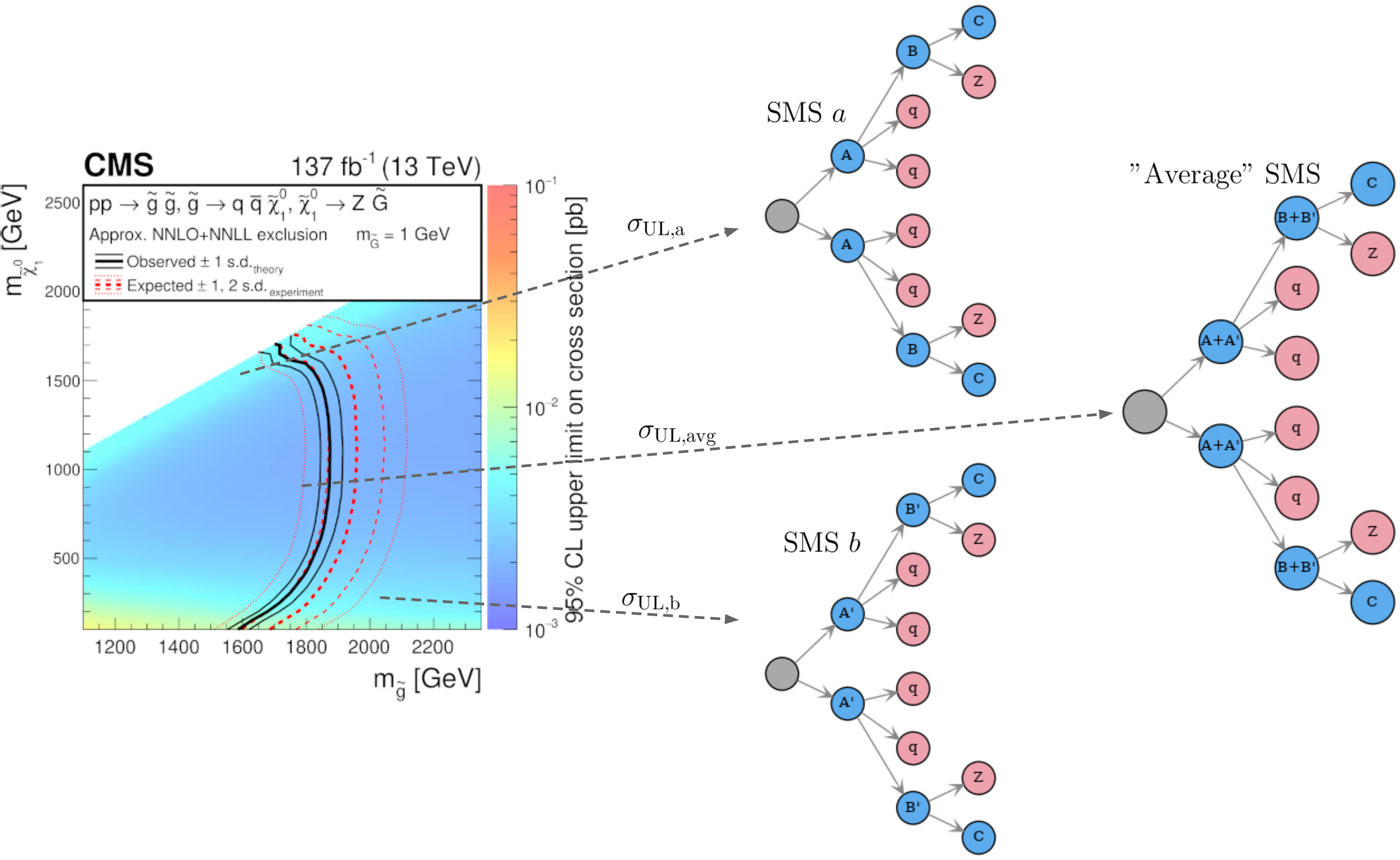
Figure 25: Example of two SMS with similar upper limit, but very distinct masses. The “average” SMS is also shown.
Hence the distance between the SMS in a given cluster and the cluster average SMS can be used as a measure to determine whether the cluster is valid or not. Furthermore, the distance between two clusters is given by the distance between the respective average SMS. The maximum allowed distance between two clusters or the cluster average SMS and the SMS within the cluster is defined by maxDist and has a default value of 0.2 (20%). The clustering algorithm is based on the following steps:
First all identical SMS (identical upper limit, masses, …) are merged, resulting in a list of average SMS.
Each SMS obtained from the previous step is assigned to its own cluster.
The pairwise distances between all clusters, \(d(c_A,c_B)\), are computed.
If \(min(d(c_A,c_B)) > maxDist \rightarrow\) stop clustering, else continue.
The pair of clusters with the smallest distance is considered for merging.
If the average SMS for the merged cluster is close in distance to all the SMS from the cluster pair \(\rightarrow\) clusters are merged
If the distance between the two clusters is greater than the maximum allowed distance, they will not be merged
Return to step 2.
The clustering of SMS is implemented by the clusterSMS method.
- 1
The comparison of the particle properties is done only for the properties which have been defined for both particles. For instance, it is often the case that the spin property is not defined for particles appearing in the database topologies, so this property will be ignored when comparing particles from the model topology and to the ones from the database topology.
- 2
In order to compare two sets of daughters (mapped to a bipartite graph) irrespective of their ordering, a maximal matching algorithm is used. Note that it is possible that the matching is not unique (i.e. \(A \leftrightarrow a, B \leftrightarrow b\) and \(A \leftrightarrow b, B \leftrightarrow a\)) and in this case the matching procedure is not deterministic.