Simplified Model Coverage

The constraints provided by SModelS are obviously limited by the variety of SMS interpretations i) provided by the experimental collaborations (or derived through recasting) and ii) implemented and validated in the database. Therefore it is interesting to identify classes of “missing topologies”, which are relevant for a given input model, but are not constrained by the SModelS database. This task is performed as a last step in SModelS, once the decomposition and the theory predictions have been computed.

During the computation of the theory predictions, each SMS topology from the decomposition which matches at least one of the simplified models in the database is marked as “covered by” the corresponding type of Experimental Result. Currently the Experimental Results are either of type prompt or displaced.1 If the same SMS is covered by both types of Experimental Results, it will be marked as covered by displaced and prompt results. If, in addition to being covered, the SMS topology also has a non-zero efficiency or upper limit (i.e. its properties fall inside the data grid of any result), it will be marked as “tested by” the corresponding type of result (prompt or displaced). Hence, after the theory predictions have been computed, the SMS topologies store information about their experimental coverage and can be classified into coverage groups.

• The coverage tool is implemented by the Uncovered class

Coverage Groups

The coverage algorithm groups all the SMS topologies into coverage groups which can be easily defined by the user (see the coverage module). Each group must define criteria for selecting topologies after the theory predictions have been computed. The default coverage groups implemented in SModelS are:

• missing (prompt): not covered by prompt-type results. This group corresponds to all SMS topologies which did not match any of the simplified models constrained by prompt Experimental Results.

• missing (displaced): not covered by displaced-type results. This group corresponds to all SMS topologies which did not match any of the simplified models constrained by displaced Experimental Results.

• missing (all): not covered by any type of result. This group corresponds to all SMS topologies which did not match any of the simplified models constrained by the database.

• outsideGrid (all): covered by at least one type of Experimental Result and not tested by any type of result. This group corresponds to all SMS topologies which matched at least one the simplified models constrained by the database, but were not tested (e.g. their masses and/or widths fall outside the efficiency or upper limit grids).

Fig. 31 schematically represents the grouping performed in coverage. Note that the coverage groups are not mutually exclusive and a give topology may fall into more than one group.

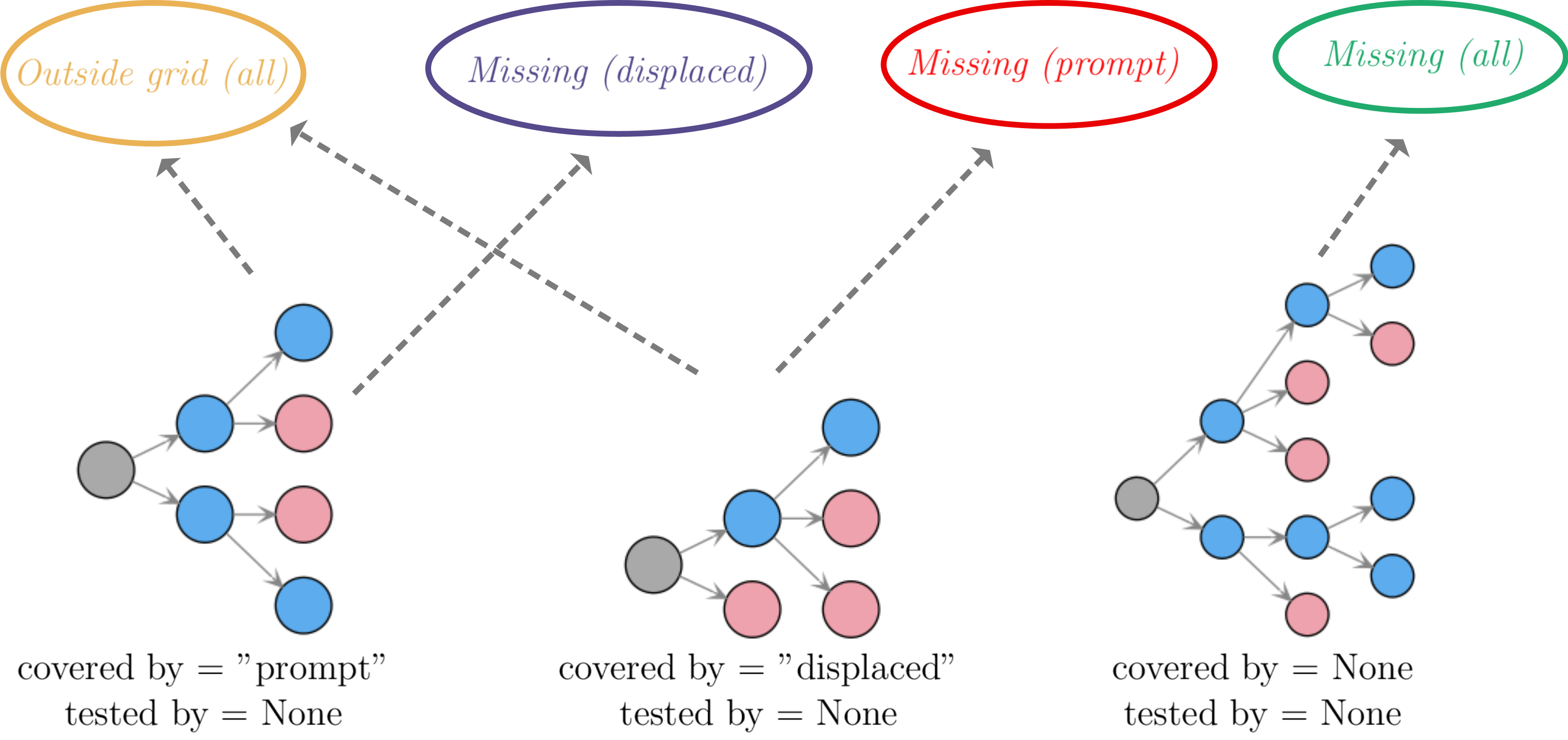
Figure 31: Schematic representation of how the SMS topologies are grouped into different coverage groups.

Besides defining which topologies should be selected, each coverage group can also specify a reweighting function for the SMS topology cross section. This is useful for the cases where the coverage group aims to represent missing topologies with prompt (or displaced) decays, so only the fraction of prompt (displaced) cross section should be extracted. The reweighting functions defined will be applied to the selected SMS in order to extract the desirable fraction of signal cross section for the group. For instance, for the default groups listed above, the following reweighting functions are defined:

• missing (prompt): \(\sigma \to \xi \times \sigma,\;\; \xi = \prod_{i=1,N-2} \mathcal{F}_{prompt}^{i} \times \prod_{i=N-2,N} \mathcal{F}_{long}^{i}\)

• missing (displaced): \(\sigma \to \xi \times \sigma,\;\; \xi = \mathcal{F}_{displaced}(any) \times \prod_{i=N-2,N} \mathcal{F}_{long}^{i}\)

• missing (all): \(\sigma \to \xi \times \sigma,\;\; \xi = 1\)

• outsideGrid (all): \(\sigma \to \xi \times \sigma,\;\; \xi = 1\)

The definition for the fraction of long-lived (\(\mathcal{F}_{long}\)) and prompt (\(\mathcal{F}_{prompt}\)) decays can be found in lifetime reweighting. The fraction \(\mathcal{F}_{displaced}(any)\) corresponds to the probability of at least one displaced decay taking place, where the probability for a displaced decay is given by \(1-\mathcal{F}_{long}-\mathcal{F}_{prompt}\).

If mass or invisible compression are turned on, SMS topologies generated by compression and their ancestors (original/uncompressed SMS) could both fall into the same coverage group. Since the total missed cross section in a given group should equal the total signal cross section not covered or tested by the corresponding type of Experimental Results, one has to avoid double counting topologies. In addition, a compressed SMS belonging to a given coverage group could combine cross sections from more than one uncompressed (original) SMS. If one of the original SMS do not belong to this coverage group (i.e. it has been covered and/or tested by the Experimental Results), its contribution to the compressed SMS cross section should be subtracted. SModelS deals with the above issues through the following steps:

• an effective “missing cross section” is computed for each SMS, which corresponds to the SMS weight subtracted of the weight of its ancestors which do not belong to the same coverage group. The effective cross section also includes the reweighting discussed above.

• All SMS topologies belonging to the same group which have a common ancestor are removed (only the SMS with largest missing cross section is kept).

• Coverage groups are implemented by the UncoveredGroup class

Final State SMS

Usually the list of SMS in each group can be considerably long, due to distinct intermediate BSM and final SM states. In order to make the list more compact, all SMS topologies are simplified to topologies where only the primary mothers and the final state particles are kept (see Fig. 32). In addition, the following SM final states particles are further combined into inclusive particles:

• \(W^+,W^- \to \mbox{W}\)

• \(\tau^+,\tau^- \to \mbox{ta}\)

• \(e^+,e^-,\mu^+,\mu^- \to \mbox{l}\)

• \(t,\bar{t} \to \mbox{t}\)

• \(u,d,s,c,\bar{u},\bar{d},\bar{s},\bar{c},g,\pi^{+,-,0} \to \mbox{jet}\)

• \(\nu_{e},\nu_{\mu},\nu_{\tau},\bar{\nu}_{e},\bar{\nu}_{\mu},\bar{\nu}_{\tau} \to \mbox{nu}\)

while the BSM particles are grouped by their signature:

• primary mothers (BSM particles produced at the PV) \(\to \mbox{anyBSM}\)

• color and electrically neutral states \(\to \mbox{MET}\)

• color neutral states with electric charge +-1 \(\to \mbox{HSCP}\)

• color triplet states with electric charge +-2/3 or +-1/3 \(\to \mbox{RHadronQ}\)

• color octet states with zero electric charge \(\to \mbox{RHadronG}\)

After the above simplification, identical simplified SMS (called Final State SMS) are combined. This procedure is illustrated in Fig. 32.

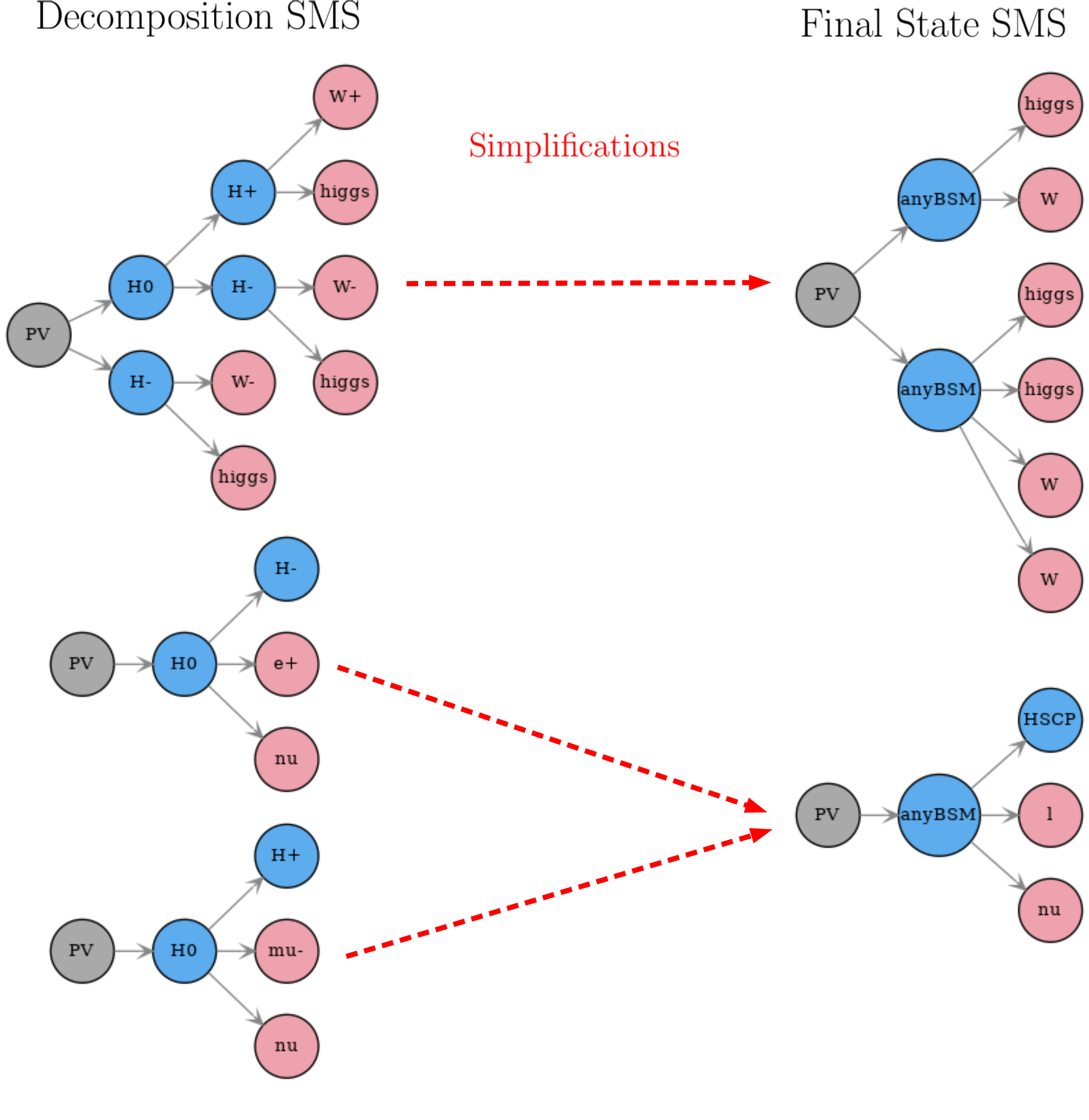
Figure 32: Schematic representation of how SMS topologies are simplified into Final State SMS and how identical Final State SMS are combined.

• Final State SMS are implemented by the FinalStateSMS class

1

Prompt results are all those which assumes all decays to be prompt and the last BSM particle to be stable (or decay outside the detector). Searches for heavy stable charged particles (HSCPs), for instance, are classified as prompt, since the HSCP is assumed to decay outside the detector. Displaced results on the other hand require at least one decay to take place inside the detector.