Simplified Model Definitions
The so-called base module contains the basic tools necessary for creating and describing simplified model topologies (SMS). Below we describe the basic concepts and language used in SModelS to describe SMS.
Simplified Model Spectrum (SMS)
The specific sequence of production and decays of BSM states is called an SMS (or SMS topology) in the SModelS language. A graph representation of an SMS is shown in Fig. 1:
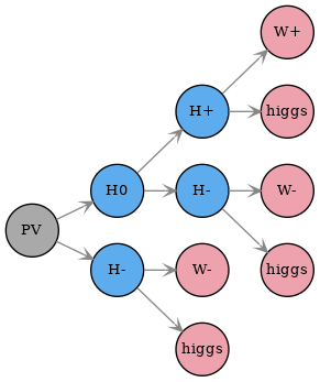
Figure 1: Graph representation of an SMS.
Each node (circle) represents a particle and the edges (connecting arrows) represents the particle decays. The first node (‘PV’) represents the primary vertex and its “daughters” are the BSM states produced in the hard scattering process. Note that the decays of SM states are not specified within the SMS, since these are assumed to be given by the SM values.
A SMS may also hold information about its corresponding weight (cross section times branching ratio times efficiency).1 The overall properties of an SMS are illustrated in Fig. 2:
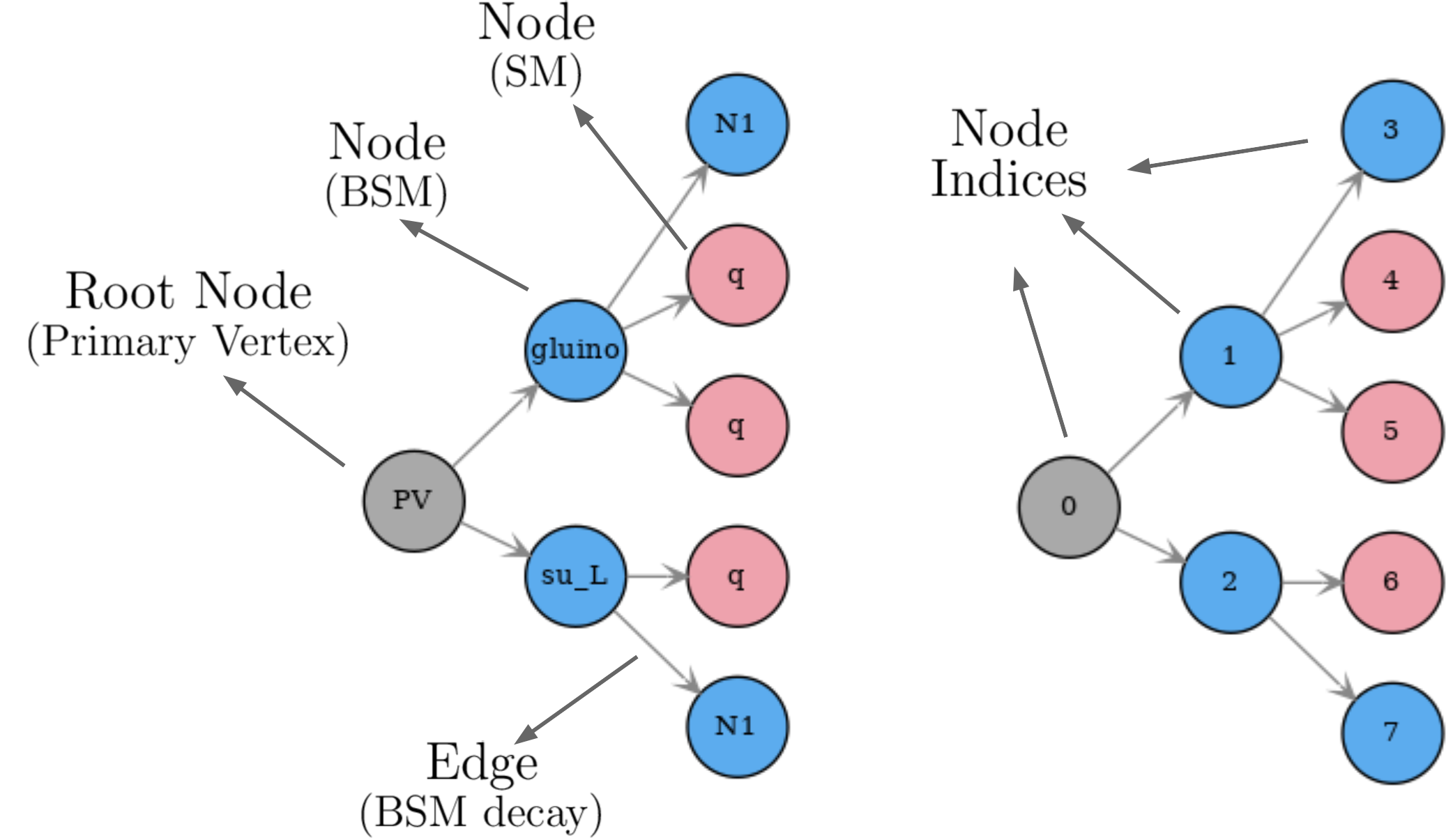
Figure 2: Illustration of the elements of an SMS graph: root node, SM and BSM nodes, edges and node indices.
SModelS works under the inherent assumption that, for collider purposes, all the essential properties of a BSM model can be encapsulated by its SMS topologies. Such an assumption is extremely helpful to cast the theoretical predictions of a specific BSM model in a model-independent framework, which can then be compared against the corresponding experimental limits. From v3.0 onwards these topologies are described by the graph structure above, with its nodes representing particles.
SMS are described by the GenericSMS Class
Particle node are described by the ParticleNode Class
Particles
The basic building block of a SMS are particles,
which can be both SM (e.g. \(W^+,higgs\) in Fig. 2)
or BSM states (e.g. \(H^0,H^+,H^-\) in Fig. 2). The particles
are mapped to nodes, which make up the SMS graph structure.
The BSM particles are defined by the input model (see model in parameters file),
while the SM particles are defined in SMparticles.py .
The BSM particles are identified by their attribute isSM = False
and they can have a flexible number of properties, such as mass, spin, electric charge, etc.
Two particles are considered equal if all their shared properties
are equal.
Generic particles are introduced by leaving one or more of their properties undefined. For instance, a particle with electric charge = -1, isSM = False, but undefined spin and mass can represent charged BSM fermions and scalars (such as charginos and charged higgses). This is useful when defining simplified models used for describing experimental results in the Database which are not sensitive to the particle’s spin. Some examples of generic particles are:
‘anyBSM’: represents any BSM state (only has isSM=False defined)
‘anySM’: represents any SM state (only has isSM=True defined)
‘MET’: represents any neutral BSM state (has isSM=False, electric charge = 0 and is a color singlet)
In addition, inclusive particles can also be created, which holds a list of particles. These can be used to described results which are inclusive over some specific set of particles. Examples are:
‘l’ for electrons, and muons,
‘L’ for electrons, muons, and taus,
‘q’ for u-, d-, and s-quarks,
‘jet’ for u-, d-, s-, c-quarks and gluons
All generic and inclusive particles used by the Database are separately defined in the databaseParticles.py file stored in the database folder or, if not found, are loaded from defaultFinalStates.py .
Particles are described by the Particle Class
Inclusive Particles are described by the MultiParticle Class
SMS Representation
A given SMS can be represented in string format using a sequence of decay patterns of the type:
X(i) > A(j),B(k),C(l)
where \(X\) represents a BSM particle, which decays to \(A,B\) and \(C\). The indices \(i,j,k,l\) refer to the node indices for the unstable particles in the SMS graph (see Fig. 2) and are needed in order to avoid ambiguities. For instance, the SMS from Fig. 2 is represented by the string:
(PV > gluino(1),su_L(2)), (gluino(1) > N1(3),q(4),q(5)), (su_L(2) > q(6),N1(7))
In order to make the output simpler, by default only the indices of decayed BSM are shown:
(PV > gluino(1),su_L(2)), (gluino(1) > N1,q,q), (su_L(2) > q,N1)
The string representation is implemented by the treeToString Method
Final states
The string representation of a SMS can be quite lengthy and it is not always fitting for some types of output. Therefore it is convenient to introduced a shortened version of its string representation, which includes only the SMS final states, i.e. the undecayed particles in the topology. For readability, the final states are group according to their primary mother produced in the topology. For instance, for a SMS described by:
PV > gluino(1),su_L(2), (gluino(1) > N1(3),q(4),q(5)), (su_L(2) > q(6),N1(7))
the corresponding final state representation is given by:
PV > (q,q,N1),(q,N1)
Although the final state representation does not uniquely identify the SMS, it is more compact and still provides information about the type of final state generated by the topology.
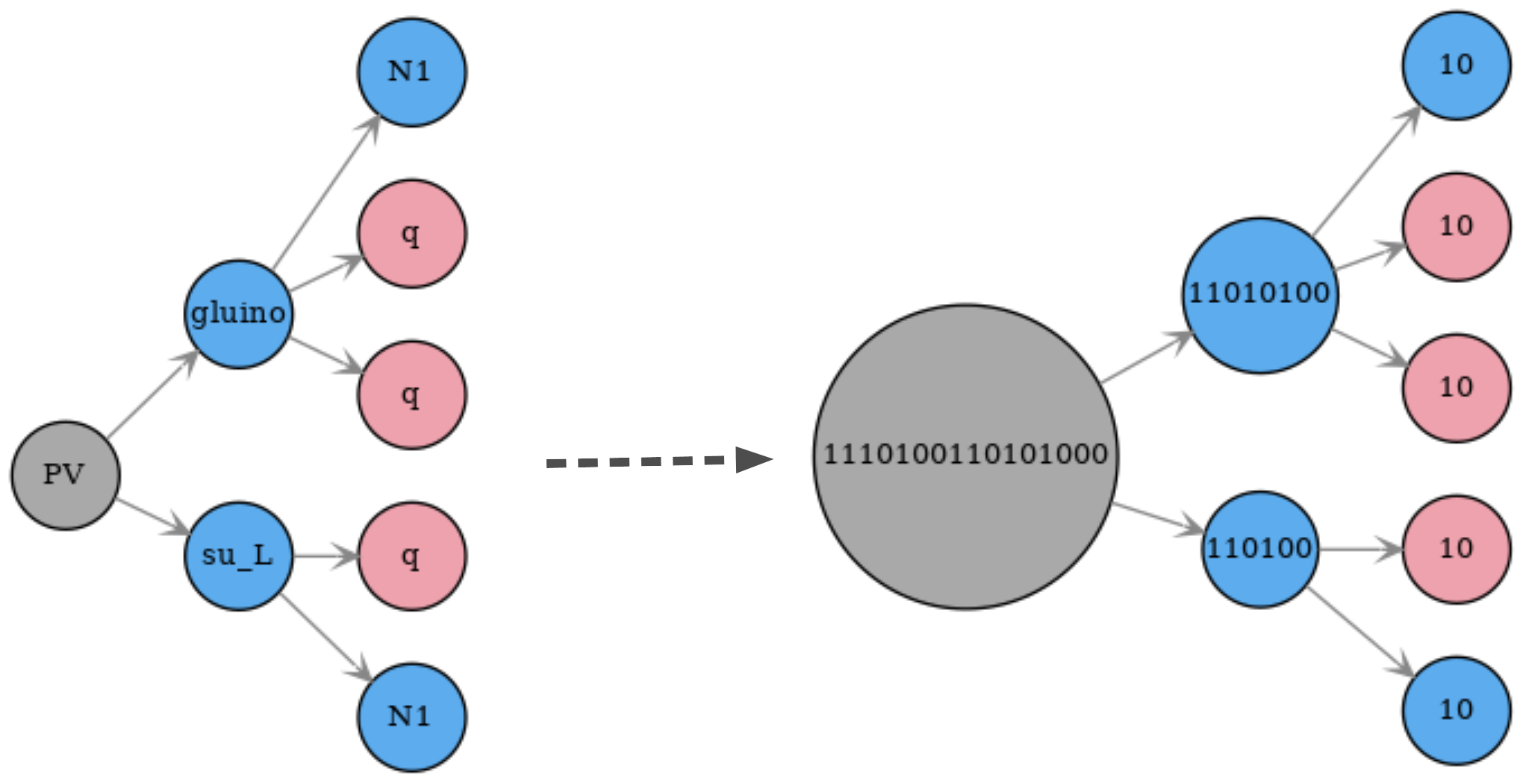
Canonical Name
It is often desirable to be able to describe the structure of a SMS topology without having to specify its particle contents. This can be extremely useful when checking if distinct SMS are equal, since if their structure differs is not needed to compare their particle nodes. This can be achieved using the canonical name (or canonical labeling) convention for rooted graphs, which assigns to each node a label according to the following rules:
each undecayed (final node) receives the label “10”
each decayed node receives the label “1<sorted labels of daughter nodes>0”
where “<sorted labels of daughter nodes>” is the joint string of the daughter nodes labels, sorted by their size. Finally the label associated to the ‘PV’ node (root node) uniquely describes the graph structure. An example is shown in Fig. 3 .