Database of Experimental Results

The information about the experimental results is stored in the SModelS Database. Below we describe both the directory and object structure of the Database and how the stored information is used within SModelS.

Database: Directory Structure

The Database is organized as files in an ordinary (UNIX) directory hierarchy, with a thin Python layer serving for the access. The overall structure of the directory hierarchy and its contents is depicted in the scheme below (click to enlarge):

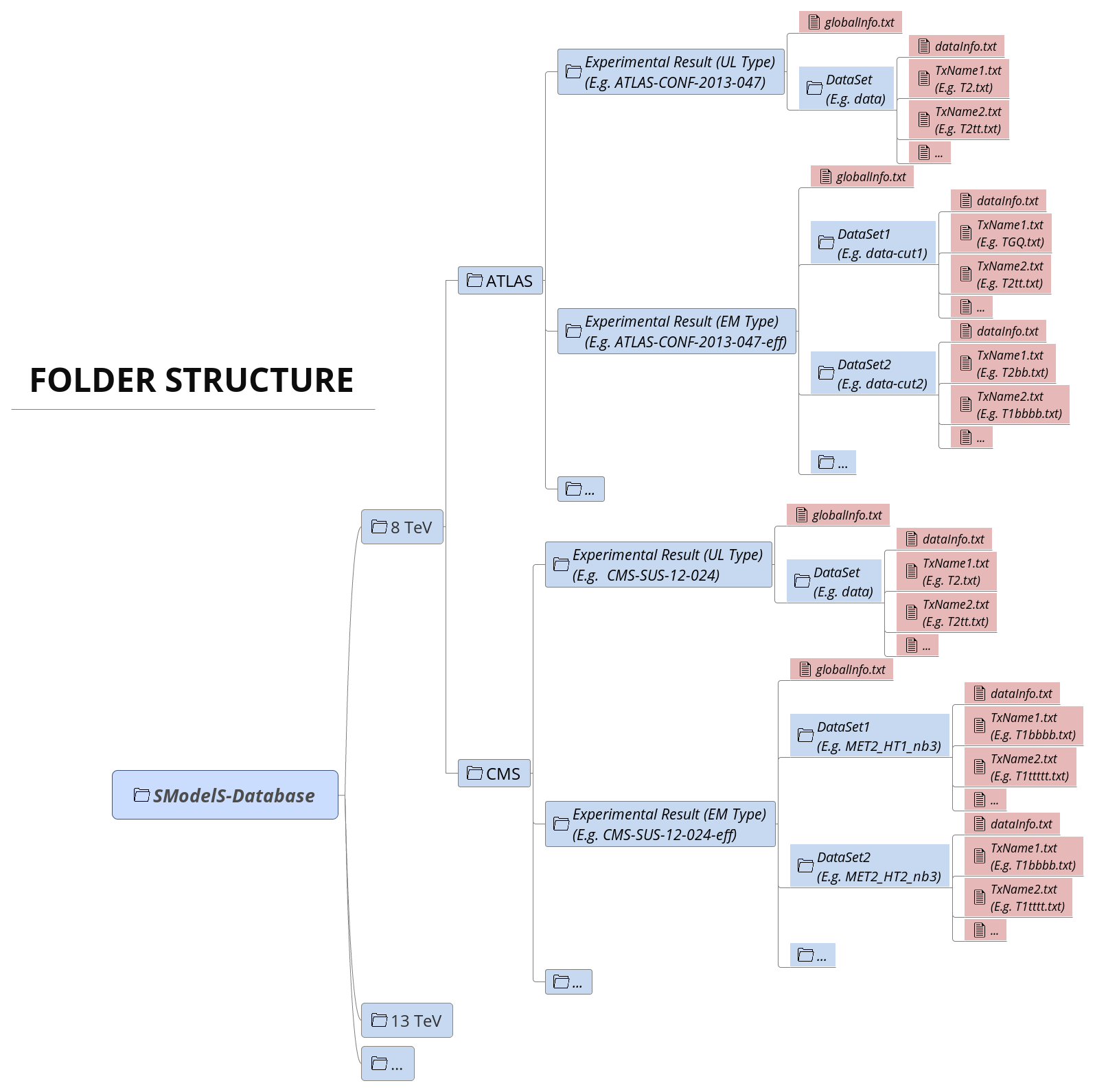
The top level directory contains a file called version with the version string of the database. At this first level, the database is organised by LHC center-of-mass energies, \(\sqrt{s}\):

8 TeV
13 TeV

The second level splits the results up between the different experiments:

8TeV/CMS/
8TeV/ATLAS/

The third level of the directory hierarchy encodes the Experimental Results:

8TeV/CMS/CMS-SUS-12-024
8TeV/ATLAS/ATLAS-CONF-2013-047
…
The Database folder is described by the Database Class

Experimental Result Folder

Each Experimental Result folder contains:

a folder for each DataSet (e.g. data)
a globalInfo.txt file

The globalInfo.txt file contains the meta information about the Experimental Result. It defines the center-of-mass energy \(\sqrt{s}\), the integrated luminosity, the id used to identify the result and additional information about the source of the data. Here is the content of CMS-SUS-12-024/globalInfo.txt as an example:

sqrts: 8.0*TeV
lumi: 19.4/fb
id: CMS-SUS-12-024
prettyName: \slash{E}_{T}+b
url: https://twiki.cern.ch/twiki/bin/view/CMSPublic/PhysicsResultsSUS12024
arxiv: http://arxiv.org/abs/1305.2390
publication: http://www.sciencedirect.com/science/article/pii/S0370269313005339
contact: Keith Ulmer <keith.ulmer@cern.ch>, Josh Thompson <joshua.thompson@cern.ch>, Alessandro Gaz <alessandro.gaz@cern.ch>
private: False
implementedBy: Wolfgang Waltenberger
lastUpdate: 2015/5/11

Experimental Result folder is described by the ExpResult Class
globalInfo files are descrived by the Info Class

Data Set Folder

Each DataSet folder (e.g. data) contains:

the Upper Limit maps for UL-type results or Efficiency maps for EM-type results (TxName.txt files)
a dataInfo.txt file containing meta information about the DataSet
Data Set folders are described by the DataSet Class
TxName files are described by the TxName Class
dataInfo files are described by the Info Class

Data Set Folder: Upper Limit Type

Since UL-type results have a single dataset (see DataSets), the info file only holds some trivial information, such as the type of Experimental Result (UL) and the dataset id (None for UL-type results). Here is the content of CMS-SUS-12-024/data/dataInfo.txt as an example:

dataType: upperLimit
dataId: None

Data Set Folder: Efficiency Map Type

For EM-type results the dataInfo.txt contains relevant information, such as an id to identify the DataSet (signal region), the number of observed and expected background events for the corresponding signal region and the respective upper limits on the fiducial cross sections. We take CMS-SUS-13-012-eff/3NJet6_1000HT1250_200MHT300/dataInfo.txt as an example:

dataType: efficiencyMap
dataId: 3NJet6_1000HT1250_200MHT300
observedN: 335
expectedBG: 305
bgError: 41
upperLimit: 5.681*fb
expectedUpperLimit: 4.585*fb

TxName Files

Each DataSet contains one or more TxName.txt files storing the bulk of the experimental result data. For UL-type results, the TxName file contains the UL maps for a given simplified model (SMS topology or sum of SMS topologies), while for EM-type results the file contains the simplified model efficiencies. In addition, the TxName files also store some meta information, such as the source of the data and the type of result (prompt or displaced). If not specified, the type will be assumed to be prompt.1 For instance, the first few lines of ATLAS-SUSY-2019-08/data/TChiWH.txt read 2:

txName: TChiWH
constraint: {(PV > anyBSM(1),anyBSM(2)), (anyBSM(1) > W,MET(3)), (anyBSM(2) > higgs,MET(4))}
condition: None
conditionDescription: None
susyProcess: pp --> neutralino_2 chargino^pm_1, neutralino_2 chargino^pm_1 --> H W lsp lsp
checked: no
figureUrl: https://atlas.web.cern.ch/Atlas/GROUPS/PHYSICS/PAPERS/SUSY-2019-08/figaux_03.png
dataUrl: https://doi.org/10.17182/hepdata.90607.v1/t17
source: ATLAS
validated: True

As seen above, the first block of data in the file contains information about the simplified model topology for which the data refers to and some additional information. The constraint field describes the SMS topology in string format (see SMS Representation).

The second block of data in the TxName.txt file contains the upper limits or efficiencies as a function of the relevant simplified model parameters:

upperLimits: [[[1.0000E+03,0.0000E+00,1.0000E+03,0.0000E+00],5.0000E-03*pb],
[[1.0000E+03,1.0000E+02,1.0000E+03,1.0000E+02],4.5000E-03*pb],
[[1.0000E+03,1.5000E+02,1.0000E+03,1.5000E+02],4.8000E-03*pb],

As seen in the example above the data is stored as arrays of BSM parameters (masses) versus upper limits:

\[[[M_1,M_2,M_3,M_4],\sigma_{UL}],...\]

The mapping between the values in the list of data points and the properties of the BSM particles appearing in the SMS topology is determined by the dataMap field stored in the TxName.txt file:

dataMap: {0:(1,'mass',GeV), 1:(3,'mass',GeV), 2:(2,'mass',GeV), 3:(4,'mass',GeV)}

The keys in dataMap are the indices of the data array (in the example above, the index goes from 0-3 referring to the four mass values), while the values are tuples containing the node index of the BSM particle (defined in the constraint string), the BSM property (‘mass’ or ‘totalwidth’) and its unit. In Fig. 26 we illustrate how the mapping works for the example above.

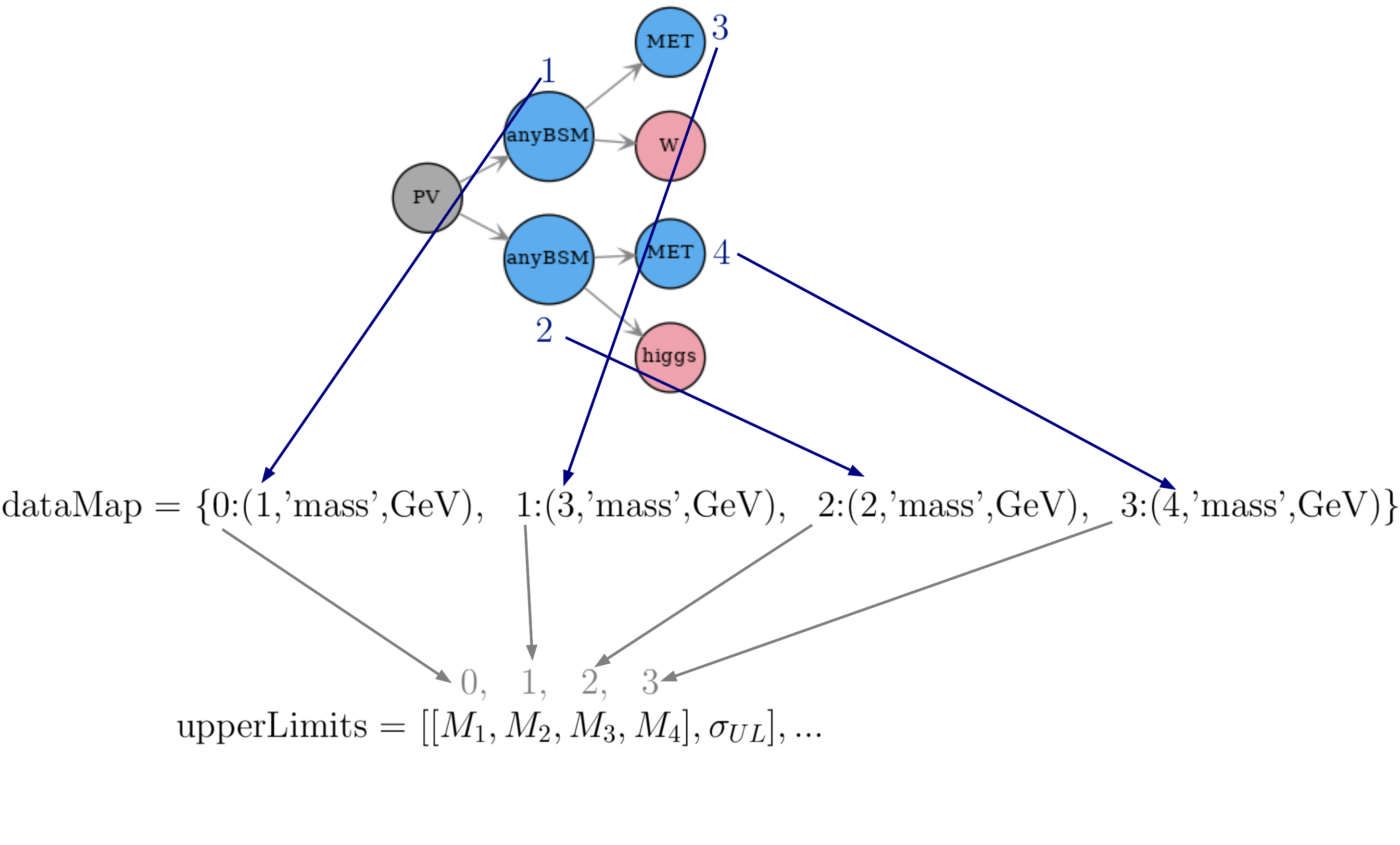
Figure 26: Schematic representation of how the values in the data are identified to properties of the SMS topology through the information stored in the dataMap field.

Results for long-lived or meta-stable particles may depend on the BSM widths as well. In this case the structure above is the same, but widths are included in the data array and are specified by the dataMap. We show one example below:

\[[[M_1,M_2,\Gamma_1,\Gamma_2],\sigma_{U}],...\]

where \(\Gamma_i\) are the relevant BSM widths. The dataMap would then take the form:

\[dataMap = \{0:(1,{\rm mass},GeV),\;\; 1:(2,{\rm mass},GeV),\;\; 2:(1,{\rm totalwidth},GeV),\;\; 3:(2,{\rm totalwidth},GeV)\}\]

In order to make the notation more compact, whenever the width dependence is not included, the corresponding decay will be assumed to be prompt and an effective lifetime reweigthing factor will be applied to the upper limits.

As discussed before (see Inclusive SMS), some analysis can be insensitive to some of the simplified model final states. In this case inclusive topologies can be described through the use of the Inclusive, anySM, *anySM strings.

Database: Object Structure

The Database folder structure is mapped to Python objects in SModelS. The mapping is almost one-to-one, with a few exceptions. Below we show the overall object structure as well as the folders/files the objects represent (click to enlarge):

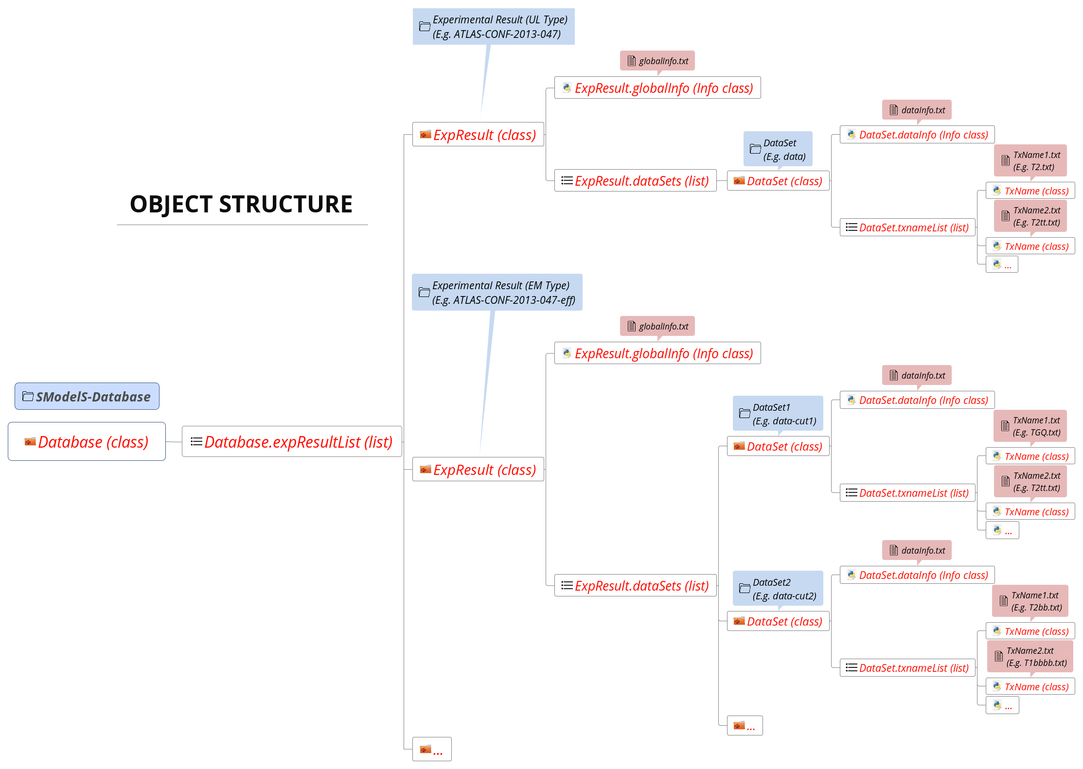
The type of Python object (Python class, Python list,…) is shown in brackets. For convenience, below we explicitly list the main database folders/files and the Python objects they are mapped to:

Database folder \(\rightarrow\) Database Class
Experimental Result folder \(\rightarrow\) ExpResult Class
DataSet folder \(\rightarrow\) DataSet Class
globalInfo.txt file \(\rightarrow\) Info Class
dataInfo.txt file \(\rightarrow\) Info Class
Txname.txt file \(\rightarrow\) TxName Class

Database: Binary (Pickle) Format

At the first time of instantiating the Database class, the text files in <database-path> are loaded and parsed, and the corresponding data objects are built. The efficiency and upper limit maps themselves are subjected to standard preprocessing steps such as a principal component analysis and Delaunay triangulation (see below). For the sake of efficiency, the entire database – including the Delaunay triangulation – is then serialized into a pickle file (<database-path>/database.pcl), which will be read directly the next time the database is loaded. If any changes in the database folder structure are detected, the python or the SModelS version has changed, SModelS will automatically re-build the pickle file. This action may take a few minutes, but it is again performed only once. If desired, the pickling process can be skipped using the option force_load = `txt’ in the constructor of Database .

The pickle file is created by the createBinaryFile method

Database: Data Processing

All the information contained in the database files is stored in the database objects. Within SModelS the information in the Database is mostly used for constraining the simplified models generated by the decomposition of the input model. Each SMS topology generated is compared to the simplified models constrained by the database and specified by the constraint entry in the TxName files. The comparison allows to identify which results can be used to test the input model. Once a matching result is found the upper limit or efficiency must be computed for the given input SMS topology. As described above, the upper limits or efficiencies are provided as function of masses and widths in the form of a discrete grid. In order to compute values for any given input SMS topology, the data has to be processed as described below.

The efficiency and upper limit maps are subjected to a few standard preprocessing steps. First, in the case of upper limits, the cross-section units are removed. Since the widths can vary over a wide range of values, they are rescaled logarithmically according to the expression:

\[\Gamma_i \to \log(1+\Gamma_i/\Gamma_0)\]

where \(\Gamma_{0} = 10^{-30}\) GeV is a rescaling factor to ensure the log is mapped to large values for the relevant width range.

Finally a principal component analysis and Delaunay triangulation (see Fig. 27) is applied over the new coordinates (unitless masses and rescaled widths) The simplices defined during triangulation are then used for linearly interpolating the transformed data grid, thus allowing SModelS to compute efficiencies or upper limits for arbitrary mass and width values (as long as they fall inside the data grid). As seen above, the width parameters are taken logarithmically before interpolation, which effectively corresponds to an exponential interpolation. If the data grid does not explicitly provide a dependence on all the widths, the computed upper limit or efficiency is then reweighted imposing the requirement of prompt decays (see lifetime reweighting for more details). This procedure provides an efficient and numerically robust way of dealing with generic data grids, including arbitrary parametrizations of the mass parameter space.

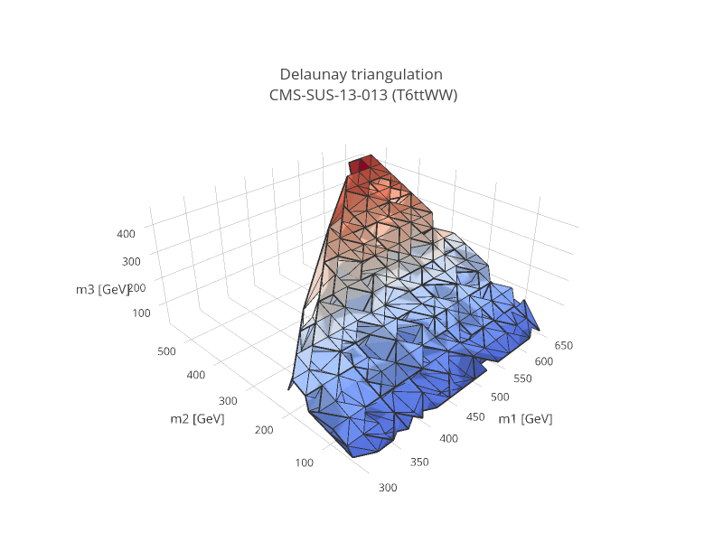
Figure 27: Illustration of the Delaunay triangulation performed over the transformed data grid for an upper limit map with three mass parameters. The colors show the upper limit values.

Lifetime Reweighting

From v2.0 onwards SModelS allows to include width dependent efficiencies and upper limits. However most experimental results do not provide upper limits (or efficiencies) as a function of the BSM particles’ widths, since usually all the decays are assumed to be prompt and the last BSM particle appearing in the cascade decay is assumed to be stable.3 In order to apply these results to models which may contain meta-stable particles, it is possible to approximate the dependence on the widths for the case in which the experimental result requires all BSM decays to be prompt and the last BSM particle to be stable or decay outside the detector. In SModelS this is done through a reweighting factor which corresponds to the fraction of prompt decays (for intermediate states) and decays outside the detector (for final BSM states) for a given set of widths.

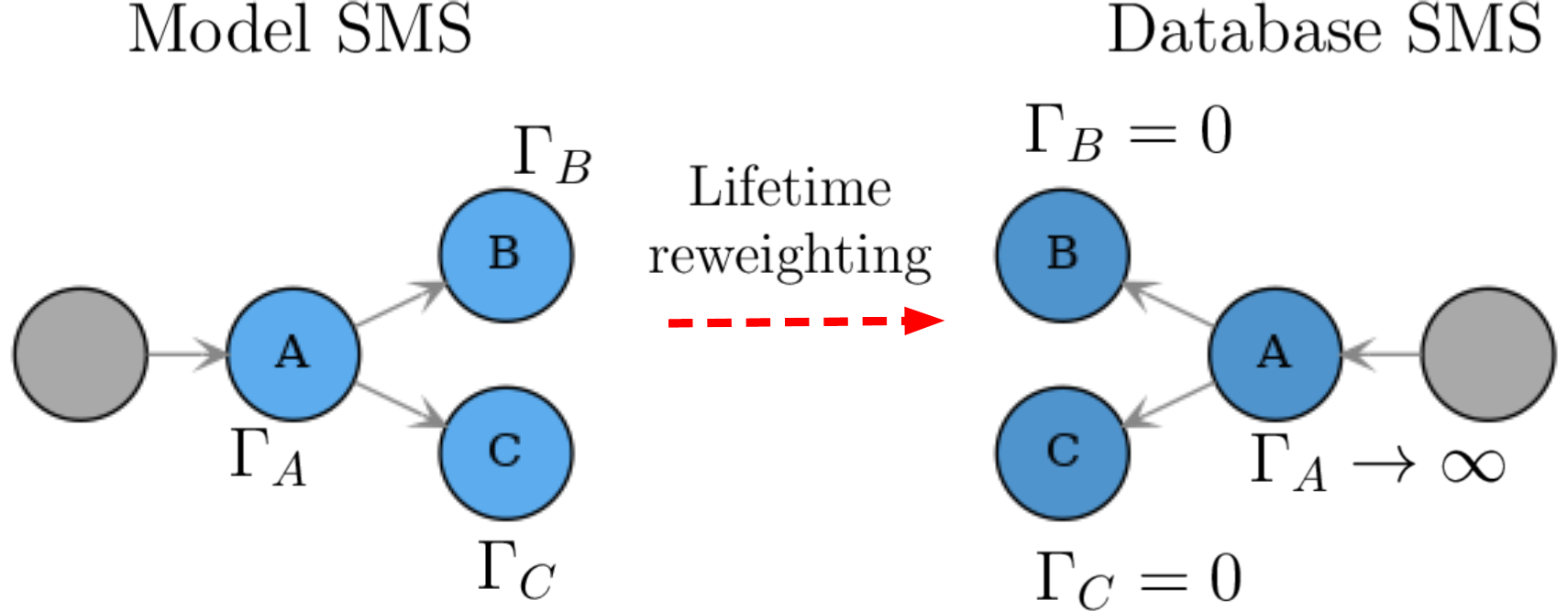
Figure 28: Representation of the lifetime reweighting applied when the experimental result assumes prompt decays of intermediate particles (e.g. \(\Gamma_A \to \infty\)) and stable final states (e.g. \(\Gamma_{B,C} = 0\)).

For instance, if an EM-type result only provides efficiencies (\(\epsilon_{prompt}\)) for prompt decays, as illustrated in Fig. 28, then, for non-zero and finite widths, an effective efficiency (\(\epsilon_{eff}\)) can be approximated by:

\[\epsilon_{eff} = \xi \times \epsilon_{prompt} \mbox{ , where }\xi = \mathcal{F}_{prompt} \left( \Gamma_{A} \right) \times \mathcal{F}_{long} \left( \Gamma_{B} \right) \times \mathcal{F}_{long} \left( \Gamma_{C} \right)\]

In the expression above \(\mathcal{F}_{prompt}(\Gamma)\) is the probability for the decay to be prompt given a width \(\Gamma\) and \(\mathcal{F}_{long}(\Gamma)\) is the probability for the decay to take place outside the detector. The precise values of \(\mathcal{F}_{prompt}\) and \(\mathcal{F}_{long}\) depend on the relevant detector size (\(L\)), particle mass (\(M\)), boost (\(\beta\)) and width (\(\Gamma\)), thus requiring a Monte Carlo simulation for each input model. Since this is not within the spirit of the simplified model approach, we approximate the prompt and long-lived probabilities by:

\[\mathcal{F}_{long} = \exp\left(- \frac{\Gamma L_{outer}}{\langle \gamma \beta \rangle}\right) \mbox{ and } \mathcal{F}_{prompt} = 1 - \exp\left(- \frac{\Gamma L_{inner}}{\langle \gamma \beta \rangle}\right),\]

where \(L_{outer}\) is the approximate size of the detector (which we take to be 10 m for both ATLAS and CMS), \(L_{inner}\) is the approximate radius of the inner detector (which we take to be 1 mm for both ATLAS and CMS). Finally, we take the effective time dilation factor to be \(\langle \gamma \beta \rangle = 1.3\) when computing \(\mathcal{F}_{prompt}\) and \(\langle \gamma \beta \rangle = 1.43\) when computing \(\mathcal{F}_{long}\). We point out that the above approximations are irrelevant if \(\Gamma\) is very large (\(\mathcal{F}_{prompt} \simeq 1\) and \(\mathcal{F}_{long} \simeq 0\)) or close to zero (\(\mathcal{F}_{prompt} \simeq 0\) and \(\mathcal{F}_{long} \simeq 1\)). Only elements containing particles which have a considerable fraction of displaced decays will be sensitive to the values chosen above. Also, a precise treatment of lifetimes is possible if the experimental result (or a theory group) explicitly provides the efficiencies as a function of the widths, as discussed above.

The above expressions allows the generalization of the efficiencies computed assuming prompt decays to models with meta-stable particles. For UL-type results the same arguments apply with one important distinction. While efficiencies are reduced for displaced decays (\(\xi < 1\)), upper limits are enhanced, since they are roughly inversely proportional to signal efficiencies. Therefore, for UL-type results, we have:

\[\sigma_{eff}^{UL} = \sigma_{prompt}^{UL}/\xi\]

Finally, we point out that for the experimental results which provide efficiencies or upper limits as a function of some (but not all) BSM widths appearing in the simplified model (see the discussion above), the reweighting factor \(\xi\) is computed using only the widths not present in the grid.

SMS Dictionary

In order to enhance the performance for the calculation of theory predictions and avoid repeated comparisons between SMS topologies generated by the decomposition and the topologies found in the database, the matching between the topologies is done in a centralized fashion. First, all the SMS topologies contained in the TxName files in the database are collected and a unique list of (sorted) SMS objects is constructed. Second, a dictionary (mapping) between the unique SMS and their equivalent topologies appearing in the TxName files is stored, as illustrated in Fig. 29.

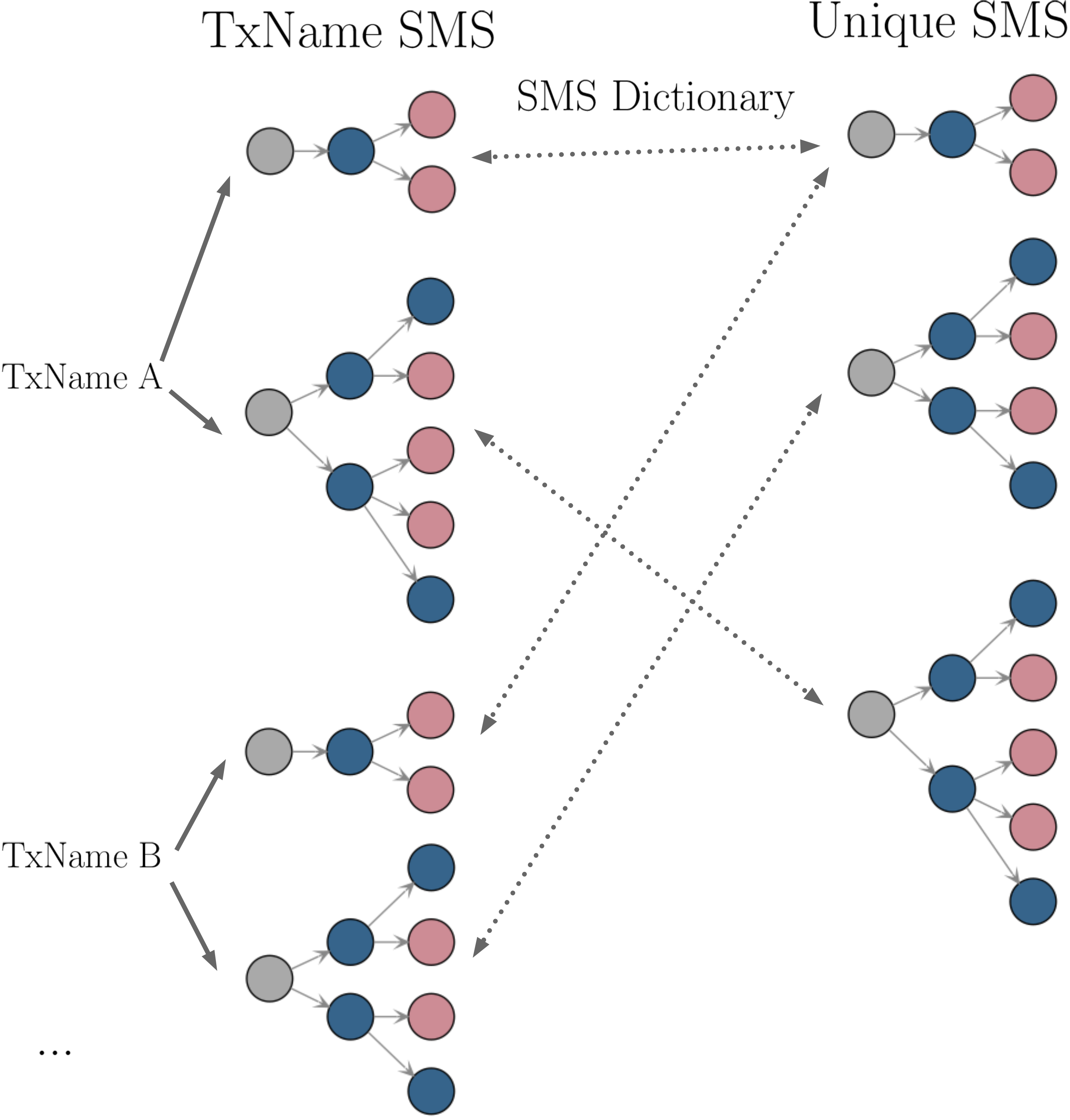
Figure 29: Representation of the SMS dictionary holding the mapping between unique SMS topologies in the SMS dictionary and the SMS topologies described in the TxName files.

The list of unique database SMS topologies is then used when matching the SMS topologies generated by the decomposition to the database. Finally, once the matching SMS have been determined, the SMS dictionary is used to translate the computed matching topologies to the original TxName topologies, as shown in Fig. 30. 4

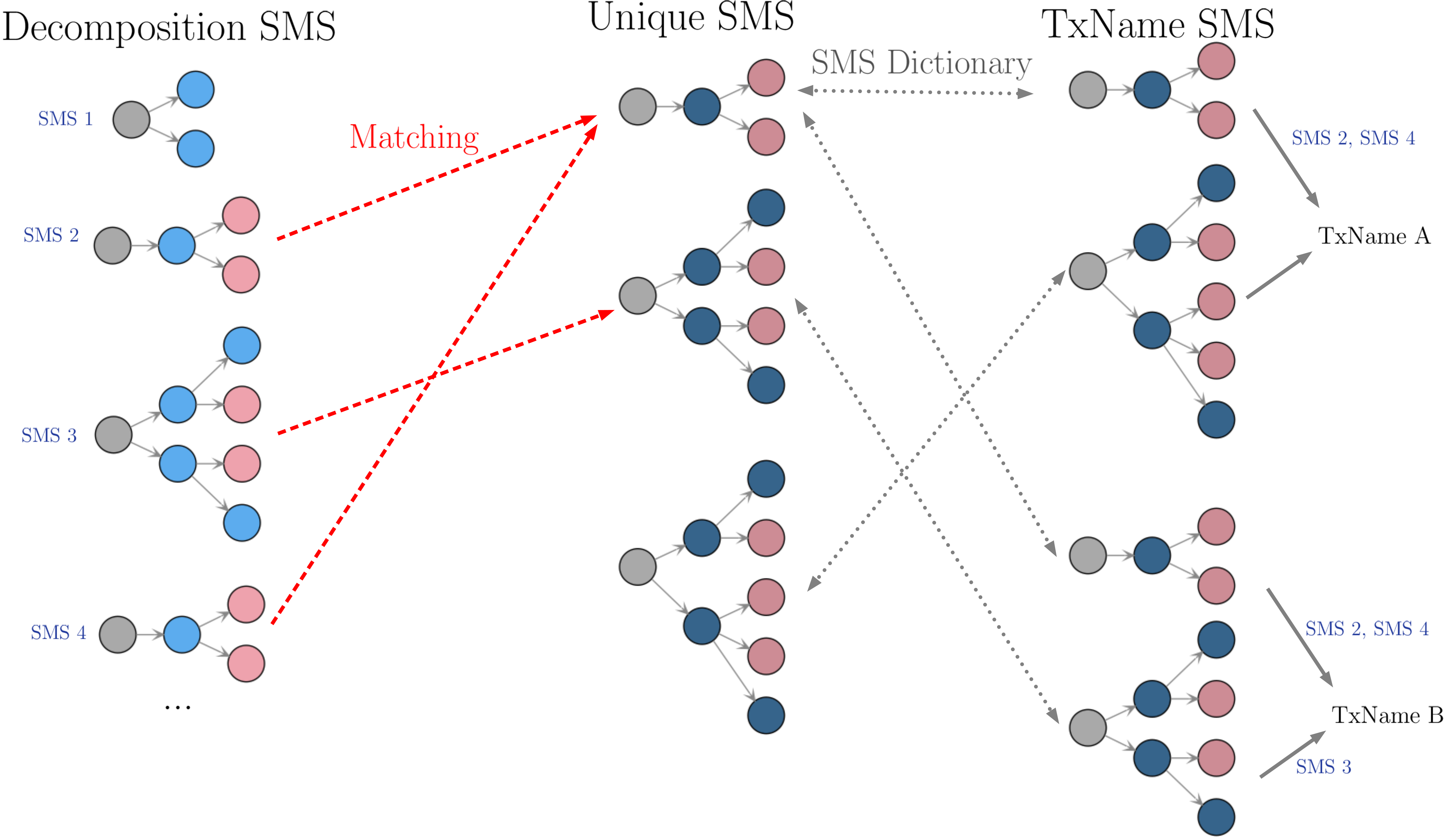
Figure 30: Schematic representation of how the matching between the SMS topologies generated by the decomposition and the SMS topologies described in the TxName files is efficiently done through the use of the SMS Dictionary.

The SMS dictionary is implemented by the ExpSMSDict class.

1: Prompt results are all those which assumes all decays to be prompt and the last BSM particle to be stable (or decay outside the detector). Searches for heavy stable charged particles (HSCPs), for instance, are classified as prompt, since the HSCP is assumed to decay outside the detector. Displaced results on the other hand require at least one decay to take place inside the detector.
2: In this example we show the metadata used for v3 onwards. For the v2 format, refer to the v2 version of this manual.
3: An obvious exception are searches for long-lived particles with displaced decays.
4: The ordering of nodes appearing in the database SMS topologies is relevant and has to be kept, since the data (ULs or EMS) assume a specific node ordering. Therefore the SMS dictionary not only identifies the unique SMS to their equivalent TxName topologies, but also how the nodes in the unique SMS are mapped to the nodes in the TxName SMS, since they could have a different ordering.