Database Definitions
The so-called experiment module contains the basic tools necessary for handling the database of experimental results. The SModelS database collects experimental results of searches from both ATLAS and CMS, which are used to compute the experimental constraints on specific models. Starting with version 1.1, the SModelS database includes two types of experimental constraints:
Upper Limit (UL) constraints: constrains on \(\sigma \times BR\) of simplified models, provided by the experimental collaborations (see UL-type results);
Efficiency Map (EM) constraints: constrains the total signal (\(\sum \sigma \times BR \times \epsilon\)) in a specific signal region. Here \(\epsilon\) denotes the acceptance times efficiency. These are either provided by the experimental collaborations or computed through recasting, e.g. with MA5 or Checkmate (see EM-type results).
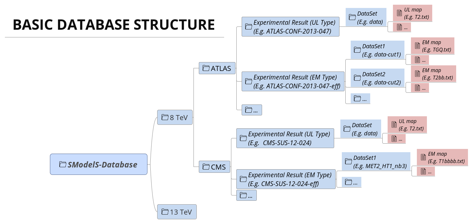
Although the two types of constraints above are very distinct, both the folder structure and the object structure of SModelS are sufficiently flexible to simultaneously handle both UL-type and EM-type results. Therefore, for both UL-type and EM-type constraints, the database obeys the following structure:
Database: collects a list of Experimental Results.
Experimental Result: each Experimental Result corresponds to an experimental preliminary result (i.e. a CONF-NOTE or PAS) or publication and contains a list of DataSets as well as general information about the result (luminosity, publication reference,…).
DataSet: a single DataSet corresponds to one signal region of the experimental note or publication.1 In case of UL-type results there is a single DataSet, usually corresponding to the best signal region or a combination of signal regions (for more details see DataSet). For EM-type results, there is one DataSet for each signal region. Each DataSet contains the Upper Limit maps for Upper Limit results or the Efficiency maps for Efficiency Map results.
Upper Limit map: contains the upper limit constraints for UL-type results. Each map contains upper limits for the signal cross-section for a single simplified model (or more precisely to a single SMS topology or sum of SMS topologies) as a function of the simplified model parameters.
Efficiency map: contains the efficiencies for EM-type results. Each map contains efficiencies for the signal for a single simplified model (or more precisely to a single SMS topologies or sum of SMS topologies) as a function of the simplified model parameters.
A schematic summary of the above structure can be seen below:
In the following sections we describe the main concepts and elements which constitute the SModelS database. More details about the database folder structure and object structure can be found in Database of Experimental Results.
Database
Each publication or conference note can be included in the database as an Experimental Result. Hence, the database is simply a collection of experimental results.
The Database is described by the Database Class
Experimental Result
An experimental result contains all the relevant information corresponding to an experimental publication or preliminary result. In particular it holds general information about the experimental analysis, such as the corresponding luminosity, center of mass energy, publication reference, etc. The current version allows for two possible types of experimental results: one containing upper limit maps (UL-type) and one containing efficiency maps (EM-type).
Experimental Results are described by the ExpResult Class
Experimental Result: Upper Limit Type
Upper Limit (UL) experimental results contain the experimental constraints on the cross section times branching ratio ( \(\sigma \times BR\) ) for Simplified Models from a specific experimental publication or preliminary result. These constraints are typically given in the format of Upper Limit maps, which correspond to 95% confidence level (C.L.) upper limit values on \(\sigma \times BR\) as a function of the respective parameter space (usually BSM masses or slices over mass planes). The UL values typically refer to the best signal region (for a given point in parameter space) or a combination of signal regions. Hence, for UL results there is a single DataSet, containing one or more UL maps. An example of a UL map is shown in Fig.4 .
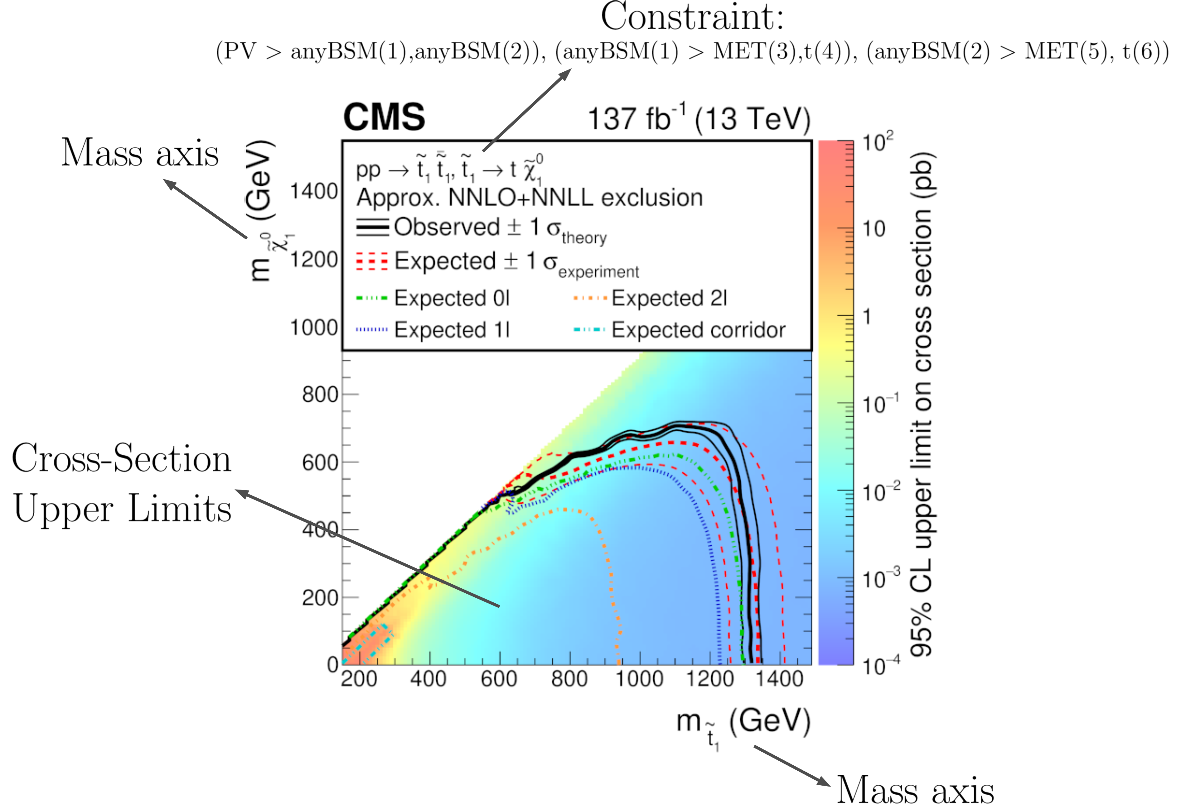
Figure 4: Example of an upper limit result and the information stored in the database.
Within SModelS, the above UL map is used to constrain the simplified model \(\tilde{t} + \tilde{t} \to \left(t+\tilde{\chi}_1^0\right) + \left(t+\tilde{\chi}_1^0\right)\). Using the SModelS string representation for simplified models, this SMS is decribed by:
(PV > anyBSM(1), anyBSM(2)) , (anyBSM(1) > MET(3),t(4)), (anyBSM(2) > MET(5),t(6))
where the integers refer to the node indices and are used internally to uniquely define the particles. Note that in the example in Fig. 4 it is assumed that the analysis is insensitive to the spin of the BSM particles and to the quantum numbers of the stop (as long as it decays to a top quark and MET), so the stops are mapped into generic BSM particles (anyBSM). A list of the database BSM particles can be found in the databaseParticles.py file in the database folder. Usually a single preliminary result/publication contains several UL maps, hence each UL-type experimental result contains several UL maps, each one constraining different simplified models (SMS topology or sum of SMS topologies). We also point out that the exclusion curve shown in the UL map above is never used by SModelS.
Upper Limit Constraint
The upper limit constraint specifies which simplified models (represented by a single SMS or a sum of SMS topologies) are being constrained by the respective UL map. For simple constraints as the one shown in Fig. 4, there is a single SMS being constrained. In some cases, however, the constraint corresponds to a sum of SMS topologies. As an example, consider the result from the ATLAS analysis in Fig. 5 :
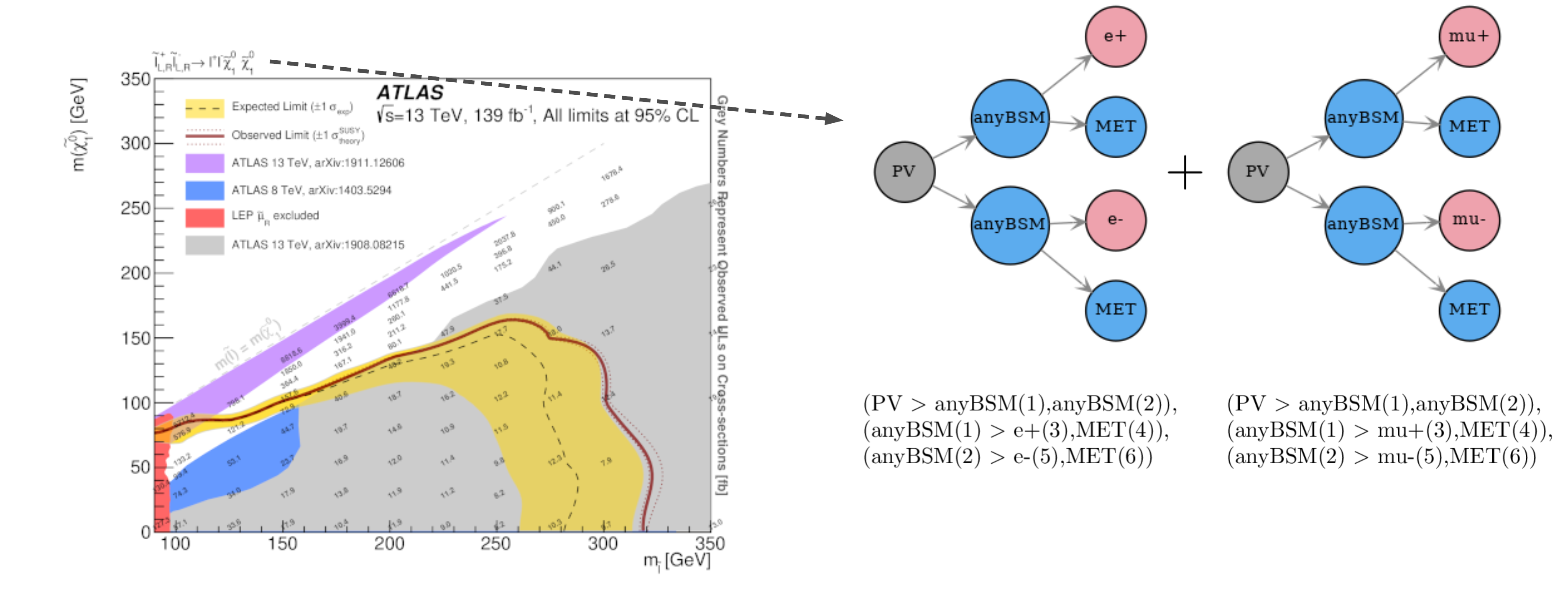
Figure 5: Example of upper limits for a sum of simplified model topologies.
As we can see, the upper limits apply to the sum of the cross sections:
In this case the UL constraint is simply:
  {(PV > anyBSM(1),anyBSM(2)), (anyBSM(1) > e+(3),MET(4)), (anyBSM(2) > e-(5),MET(6))}

+ {(PV > anyBSM(1),anyBSM(2)), (anyBSM(1) > mu+(3),MET(4)), (anyBSM(2) > mu-(5),MET(6))}
where it is understood that the sum runs over the weights of the respective SMS. Note that curly brackets were introduced in order delimit individual SMS topologies.
Note that the sum can be over particle charges, flavors or more complex combinations of simplified models. However, almost all experimental results sum only over SMS sharing a common structure (or common canonical name).
Finally, in some cases the UL constraint assumes specific contributions from each individual simplified model. For instance, in Fig. 5 it is implicitly assumed that both the electron and muon SMS contribute equally to the total cross section. Hence these conditions must also be specified along with the constraint, as described in UL conditions.
Upper Limit Conditions
When the analysis constraints are non-trivial (refer to a sum of SMS), it is often the case that there are implicit (or explicit) assumptions about the contribution of each simplified model. For instance, in Fig. 5, it is implicitly assumed that each lepton flavor contributes equally to the summed cross section:
Therefore, when applying these constraints to general models, one must also verify if these conditions are satisfied. Once again we can express these conditions using the string representation of simplified models:
{(PV > anyBSM(1),anyBSM(2)), (anyBSM(1) > e+(3),MET(4)), (anyBSM(2) > e-(5),MET(6))}
= {(PV > anyBSM(1),anyBSM(2)), (anyBSM(1) > mu+(3),MET(4)), (anyBSM(2) > mu-(5),MET(6))}
where it is understood that the condition refers to the weights of the respective simplified models.
In several cases it is desirable to relax the analysis conditions, so the analysis upper limits can be applied to a broader spectrum of models. Once again, for the example mentioned above, it might be reasonable to impose instead:
{(PV > anyBSM(1),anyBSM(2)), (anyBSM(1) > e+(3),MET(4)), (anyBSM(2) > e-(5),MET(6))}
<= {(PV > anyBSM(1),anyBSM(2)), (anyBSM(1) > mu+(3),MET(4)), (anyBSM(2) > mu-(5),MET(6))}
The departure from the exact condition can then be properly quantified and one can decide whether the analysis upper limits are applicable or not to the model being considered. Concretely, SModelS computes for each condition a number between 0 and 1, where 0 means the condition is exactly satisfied and 1 means it is maximally violated. Allowing for a \(20\%\) violation of a condition corresponds approximately to a ‘’condition violation value’’ (or simply condition value) of 0.2. The condition values are given as an output of SModelS, so the user can decide what are the maximum acceptable values (see maxcond in the parameters file).
Experimental Result: Efficiency Map Type
Efficiency maps correspond to a grid of simulated acceptance times efficiency ( \(A \times \epsilon\) ) values for a specific signal region. In the following we will refer to \(A \times \epsilon\) simply as efficiency and denote it by \(\epsilon\). Furthermore, additional information, such as the luminosity, number of observed and expected events, etc is also stored in an EM-type result.
Another important difference between UL-type results and EM-type results is the existence of several signal regions, which in SModelS are mapped to DataSets. While UL-type results contain a single DataSet (‘’signal region’’), EM results hold several DataSets, one for each signal region (see the database scheme above). Each DataSet contains one or more efficiency maps, one for each SMS. The efficiency map is usually a function of the BSM masses (or masses and widths) appearing in the element, as shown in Fig. 6:
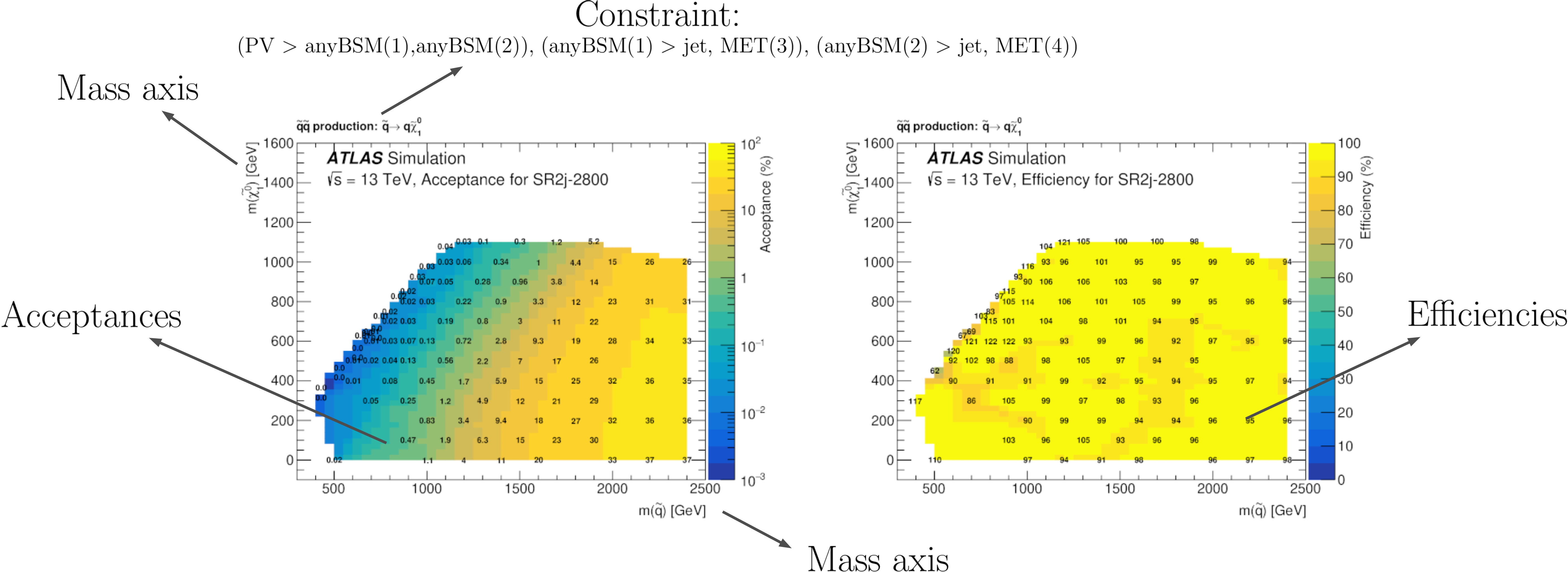
Figure 6: Example of an EM-type result. Note that only the product \(\mathcal{A} \times \epsilon\) is used by SModelS.
In order to use a language similar to the one used in UL-type results, the description of SMS for which the efficiencies correspond still is called constraint.
Although efficiencies are most useful for EM-type results, their concept can also be extended to UL-type results. For the latter, the efficiency for a given SMS is either 1, if the simplified model appears in the UL constraint, or 0, otherwise. Although trivial, this extension allows for a unified treatment of EM-type results and UL-type results (see Theory Predictions for more details).
Data Sets
Data sets are a way to conveniently group efficiency maps corresponding to the same signal region. As discussed in UL-type results, data sets are not necessary for UL-type results, since in this case there is a single ‘’signal region’’. Nonetheless, data sets are also present in UL-type results in order to allow for a similar structure for both EM-type and UL-type results (see database scheme).
For UL-type results the data set contains the UL maps as well as some basic information, such as the type of Experimental Result (UL). On the other hand, for EM-type results, each data set contains the EM maps for the corresponding signal region as well as some additional information: the observed and expected number of events in the signal region, the signal upper limit, etc. In the folder structure shown in database scheme, the upper limit maps and efficiency maps for each SMS (or sum of SMS) are stored in files labeled according to the TxName convention.
Data Sets are described by the DataSet Class
TxName Convention
Since using the string notation to describe the simplified models appearing in the upper limit or efficiency maps can be rather lengthy, it is useful to define a shorthand notation for the constraints. SModelS adopts a notation based on the CMS SMS conventions, where each specific constraint is labeled as T<constraint name>, which we refer as TxName. For instance, the TxName corresponding to the constraint in Fig. 6 is T2. A complete list of TxNames can be found here.
Upper limit and efficiency maps are described by the TxName Class
More details about the database folder structure and object structure can be found in Database of Experimental Results.
Inclusive SMS
The experimental searches are often inclusive over the final states considered, as illustrated by the sum over light lepton flavors in Fig. 5. Also, many searches are not strongly sensitive to the quantum numbers of the promptly decaying BSM particles. Finally, some searches are very inclusive over the final states as long as the required target object/particle is present in the signal. All these different levels of inclusiveness need to be represented by the SMS topologies appearing in the constraints and the following objects can be used when describing inclusive constraints:
Inclusive particles/labels: these can be used to describe several particles which are considered equivalent for the experimental search. For instance, jets can be represented by an inclusive particle, which equals any light quark flavor or a gluon (\(jet = u,d,s,c,g\)). A fully inclusive label can also be used to describe any BSM state (\(anyBSM\)) or any SM state (\(anySM\)). Finally any BSM or SM particle is represented by \(*\). An example of the use of inclusive labels is shown in Fig. 7.
Inclusive number of SM particles: some inclusive searches allow for an arbitrary number of SM particles in the final once they satisfy some requirements. The arbitrary number of SM particles is represented by \(*anySM\). One example is the search for disappearing tracks, which is insensitive to the the decay of the long-lived particle, as long as the SM states from the decay are soft and the BSM state is invisible, as represented in Fig. 8.
Inclusive topologies: in highly inclusive searches even the topology of the SMS is arbitrary, as long as the final states satisfy some loose requirements. This case is described by an “inclusive” particle (node), which represents any arbitrary cascade decay. For example, any cascade decay may be allowed as long as there are only SM particles appearing as final states or invisible BSM states. One example is the search for heavy stable charged particles, which is fairly insensitive to the extra activity in the event as long as a heavy particle charged particle is also present, as illustrated in Fig. 9.
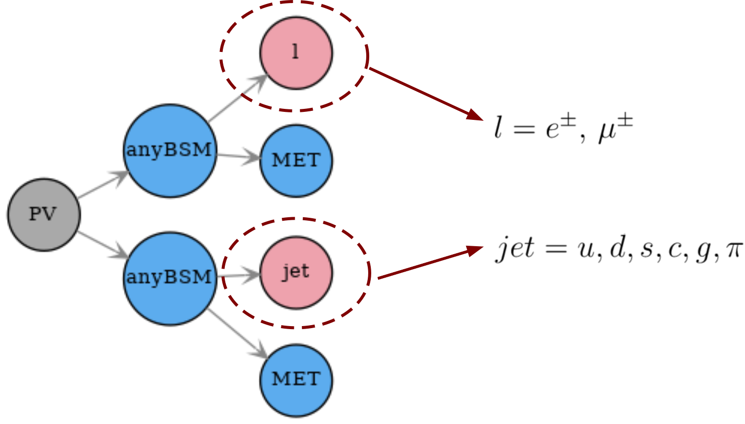
Figure 7: Example of how inclusive labels can be used in SMS topologies describing inclusive final states. In the example above \(l\) represents any light charged lepton (electrons, muons) and \(jet\) represents any light quark, gluon or pions.
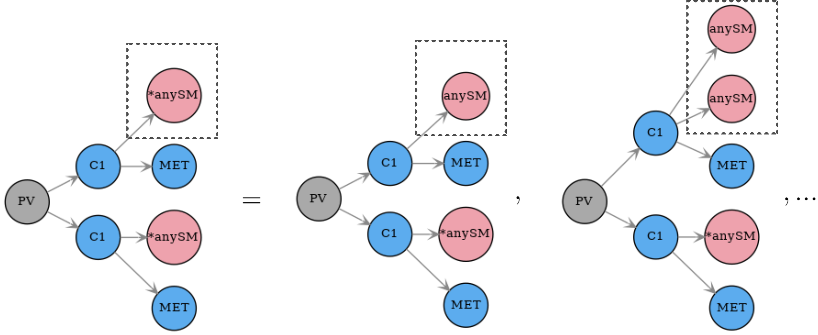
Figure 8: Example of how SMS topologies with an arbitrary number of SM final states is represented within SModelS. The particle (node) \(*anySM\) describes any number of SM final states appearing in the \(C1\) decay.
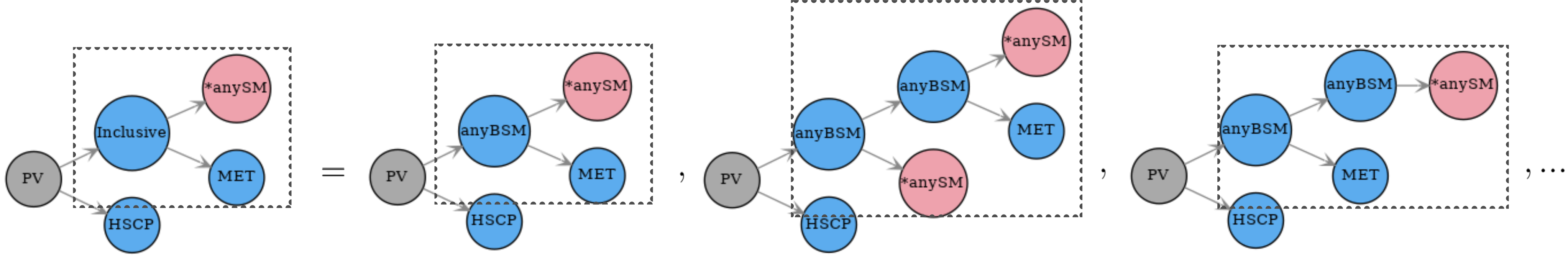
Figure 9: Example of how inclusive topologies are represented within SModelS. The particle (node) \(Inclusive\) describes arbitrary cascade decays which lead to one BSM invisible final state (\(MET\)) and an arbitrary number of SM final states (\(*anySM\)).
- 1
The name Data Set is used instead of signal region because its concept is slightly more general. For instance, in some EM-type results a DataSet may not correspond to an aggregated signal region, while for UL-type results it may correspond to a combination of all signal regions.