Confronting Predictions with Experimental Limits
Once the relevant signal cross sections (or theory predictions) have been computed for the input model, these must be compared to the respective upper limits. The upper limits for the signal are stored in the SModelS Database and depend on the type of Experimental Result: UL-type or EM-type.
In the case of a UL-type result, the theory predictions typically consist of a list of signal cross sections (one for each cluster) for the single data set (see Theory Predictions for Upper Limit Results for more details). Each theory prediction must then be compared to its corresponding upper limit. This limit is simply the cross section upper limit provided by the experimental publication or conference note and is extracted from the corresponding UL map (see UL-type results).
For EM-type results there is a single cluster for each data set (or signal region), and hence a single signal cross section value. This value must be compared to the upper limit for the corresponding signal region. This upper limit is easily computed using the number of observed and expected events for the data set and their uncertainties and is typically stored in the Database. Since most EM-type results have several signal regions (data sets), there will be one theory prediction/upper limit for each data set. By default SModelS keeps only the best data set, i.e. the one with the largest ratio \(r_\mathrm{exp}=(\mathrm{theory\,prediction})/(\mathrm{expected\, limit})\). (See below for combination of signal regions) Thus each EM-type result will have a single theory prediction/upper limit, corresponding to the best data set (based on the expected limit). If the user wants to have access to all the data sets, the default behavior can be disabled by setting useBestDataset=False in theoryPredictionsFor (see Example.py).
The procedure described above can be applied to all the Experimental Results in the database, resulting in a list of theory predictions and upper limits for each Experimental Result. A model can then be considered excluded by the experimental results if, for one or more predictions, we have theory prediction \(>\) upper limit 1.
The upper limits for a given UL-type result or EM-type result can be obtained using the getUpperLimitFor method
Likelihood Computation
In the case of EM-type results, additional statistical information about the constrained model can be provided by the SModelS output. Most importantly, we can compute a likelihood, which describes the plausibility of a signal strength \(\mu\) given the data \(D\):
Here, \(\theta\) denotes the nuisance parameter that describes the variations in the signal and background contribtions due to systematic effects, \(s\) is the number of predicted signal events.
If no information about the correlation of signal regions is available (or if its usage is turned off, see Using SModelS), we compute a simplified likelihood for the most sensitive (a.k.a. best) signal region, i.e. the signal region with the highest \(r_\mathrm{exp}=(\mathrm{theory\,prediction})/(\mathrm{expected\, limit})\), following the procedure detailed in CMS-NOTE-2017-001.
This means we assume \(p(\theta)\) to follow a Gaussian distribution centered around zero and with a variance of \(\delta^2\), whereas \(P(D)\) corresponds to a counting variable and is thus properly described by a Poissonian. The complete likelihood thus reads:
where \(n_{obs}\) is the number of observed events in the signal region. From this likelihood we compute a 95% confidence level limit on \(\mu\) using the \(CL_s\) (\(CL_{sb}/CL_{b}\)) limit from the test statistic \(q_\mu\), as described in Eq. 14 in G. Cowan et al., Asymptotic formulae for likelihood-based tests. We then search for the value \(CL_s = 0.95\) using the TOMS algorithm available through the scipy optimize library. 2 This is used for the computation the observed and expected \(r\) values.
- In addition, SModelS reports for each EM-type result :
the likelihood for the hypothezised signal, \(\mathcal{L}_{\mathrm{BSM}}\) given by \(\mu=n_{\mathrm{signal}}\),
the likelihood for the SM, \(\mathcal{L}_{\mathrm{SM}}\) given by \(\mu=0\), and
the maximum likelihood \(\mathcal{L}_{\mathrm{max}}\) obtained by setting \(\mu=n_{\mathrm{obs}}-b\).
The values for \(n_{\mathrm{obs}}\), \(b\) and \(\delta_{b}\) are directly extracted from the data set (coined observedN, expectedBG and bgError, respectively), while \(n_{\mathrm{signal}}\) is obtained from the calculation of the theory predictions. A default 20% systematical uncertainty is assumed for \(n_{\mathrm{signal}}\), resulting in \(\delta^2 = \delta_{b}^2 + \left(0.2 n_{\mathrm{signal}}\right)^2\).
We note that in the general case analyses may be correlated, so the likelihoods from different analyses cannot straightforwardly be combined into a global one. Therefore, for a conservative interpretation, only the result with the best expected limit should be used. Moreover, for a statistically rigorous usage in scans, it is recommended to check that the analysis giving the best expected limit does not wildly jump within continuous regions of parameter space that give roughly the same phenomenology.
Finally, note that in earlier SModelS versions, a \(\chi^2\) value, defined as \(\chi^2=-2 \ln \frac{\mathcal{L}_{\mathrm{BSM}}}{\mathcal{L}_{\mathrm{max}}}\) was reported instead of \(\mathcal{L}_{\mathrm{max}}\) and \(\mathcal{L}_{\mathrm{SM}}\). From v2.1 onwards, the definition of a test statistic for, e.g., likelihood ratio tests, is left to the user.
The likelihood for a given EM-type result is computed using the likelihood method
The maximum likelihood for a given EM-type result is computed using the lmax method
Combination of Signal Regions
The likelihoods from individual signal regions can be combined, if the experimental analysis provides the required information about the correlation between distinct signal regions. Currently two approaches are available, depending on which type of information is provided by the experimental collaborations. When using runSModelS.py, the combination of signal regions is turned on or off with the parameter options:combineSRs, see parameter file. Its default value is False, in which case only the result from the best expected signal region (best SR) is reported. If combineSRs = True, the combined result is shown instead.
Simplified Likelihood Approach
The first approach is applicable when information about the (background) correlations is available in the form of a covariance matrix. Some CMS analyses provides such matrix together with the efficiency maps. The usage of such covariance matrices is implemented in SModelS v1.1.3 onwards, following as above the simplified likelihood approach described in CMS-NOTE-2017-001.
Since CPU performance is a concern in SModelS, we try to aggregate the official results, which can comprise >100 signal regions, to an acceptable number of aggregate regions. Here acceptable means as few aggregate regions as possible without loosing in precision or constraining power. The CPU time scales roughly linearly with the number of signal regions, so aggregating e.g. from 80 to 20 signal regions means gaining a factor 4 in computing time.
Under the assumptions described in CMS-NOTE-2017-001, the likelihood for the signal hypothesis when combining signal regions is given by:
where the product is over all \(N\) signal regions, \(\mu\) is the overall signal strength, \(s_i^r\) the signal strength in each signal region and \(V\) represents the covariance matrix. Note, however, that unlike the case of a single signal region, we do not include any signal uncertainties, since this should correspond to a second-order effect.
As above, we compute a 95% confidence level limit on \(\mu\) using the \(CL_s\) (\(CL_{sb}/CL_{b}\)) limit from the test statistic \(q_\mu\), as described in Eq. 14 in G. Cowan et al., Asymptotic formulae for likelihood-based tests. We then search for the value \(CL_s = 0.95\) using the using the TOMS algorithm available through the scipy optimize library. 2 Note that the limit computed through this procedure applies to the total signal yield summed over all signal regions and assumes that the relative signal strengths in each signal region are fixed by the signal hypothesis. As a result, the above limit has to be computed for each given input model (or each theory prediction), thus considerably increasing CPU time.
In the figure below we show the constraints on the simplified model T2bbWWoff when using the best signal region (left), all the 44 signal regions considered in CMS-PAS-SUS-16-052 (center) and the aggregated signal regions included in the SModelS database (right). As we can see, while the curve obtained from the combination of all 44 signal regions is much closer to the official exclusion than the one obtained using only the best SR. Finally, the aggregated result included in the SModelS database (total of 17 aggregate regions) similarly matches the official result, but considerably reduces the run time.
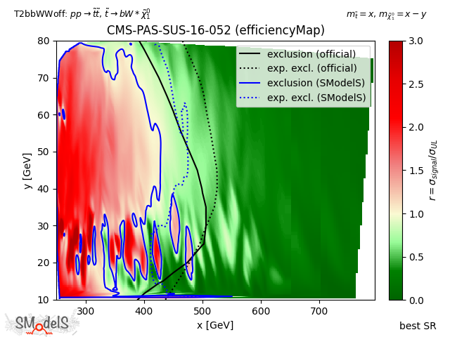
Best signal region
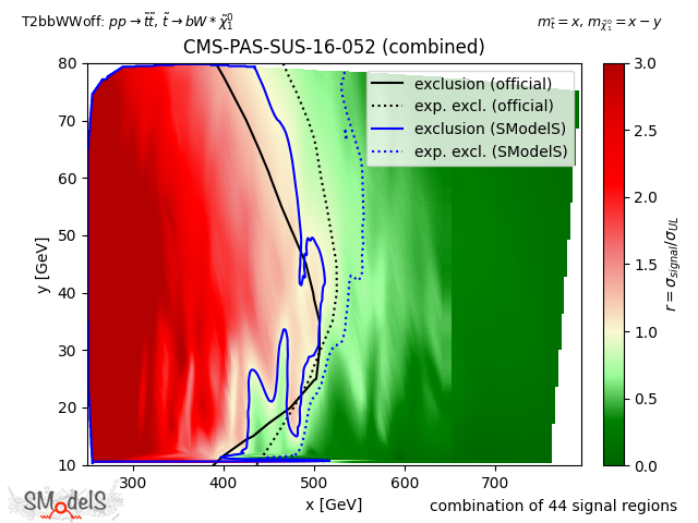
44 signal regions
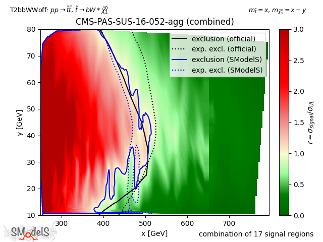
17 aggregate regions
Figure: Comparison of exclusion curves for CMS-PAS-SUS-16-052 using only the best signal region (left), the combination of all 44 signal regions (center), and the combination of 17 aggregate signal regions (right).
Simplified Likelihood v2
From SModelS v2.3 on, simplified likelihoods with a skew (a.k.a. SLv2), as described in The Simplified Likelihood Framework paper, are supported. The simplified likelihood above (which we now call SLv1) is extended to account for a skewness in the nuisances:
Here, \(\rho\) denotes the correlation matrix, and \(a_i\), \(b_i\), and \(c_i\) are functions of the background expectations, and their second and third statistical momenta. In order for a result to be declared SLv2 in SModelS, third statistical momenta must be provided in addition to background expectations and their errors.
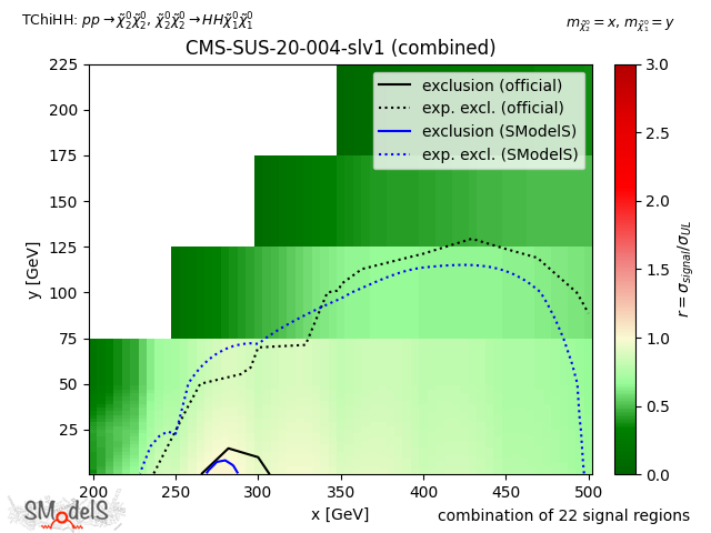
The figure below shows a comparison for TChiHH of CMS-SUS-20-004, using a simplified likelihood but ignoring the third momenta, i.e. SLv1 (left), and a simplified likelihood result v2 (right).
SLv1
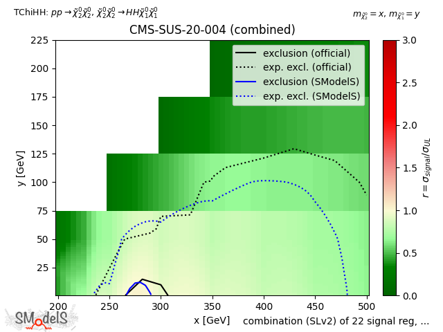
SLv2
Figure: Comparison of CMS-SUS-20-004 using SLv1 (left), and SLv2 (right).
Full Likelihoods (pyhf) Approach
In early 2020, following ATL-PHYS-PUB-2019-029, ATLAS has started to provide full likelihoods for results with full Run 2 luminosity (139/fb), using a JSON serialisation of the likelihood. This JSON format describes the HistFactory family of statistical models, which is used by the majority of ATLAS analyses. Thus background estimates, changes under systematic variations, and observed data counts are provided at the same fidelity as used in the experiment.
SModelS supports the usage of these JSON likelihoods from v1.2.4 onward via an interface to the pyhf package, a pure-python implementation of the HistFactory statistical model. This means that for EM-type result from ATLAS, for which a JSON likelihood is available and when the combination of signal regions is turned on, the evaluation of the likelihood is relegated to pyhf. Internally, the whole calculation is based on the asymptotic formulas of Asymptotic formulae for likelihood-based tests of new physics, arXiv:1007.1727.
By default, the control regions (CRs) are removed from the statistical model. The possibility to prevent this has been added with SModelS v.2.2.0 through the includeCRs flag in the globalInfo.txt files. From v3.0.0 onward, SModelS can emulate signal leaking into the CRs if efficiency maps are provided for them. The statistical treatment of CRs is identical to the one of SRs, except that the former are not allowed to individually constrain the tested model. If includeCRs = False in the globalInfo.txt file, the CRs as well as the leaking signals are removed from the statistical model. Additionally, v3.0.0 added the possibility to incorporate signal uncertainty within the statistical model. When a value is provided in the signalUncertainty field of the globalInfo.txt file, each nominal signal of each bin of each channel (CRs as well as SRs) can be modified through an additive nuisance parameter constrained by a Gaussian (more precisely, it is done through pyhf “correlated shape” modifiers). These choices have been made at the level of the analysis implementation and are not directly accessible to the user.
The figure below exemplifies how the constraints improve from using the best signal region (left) to using the full likelihood (right).
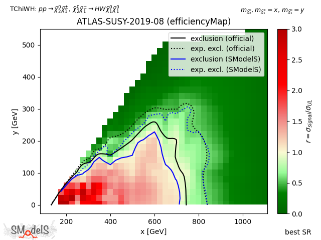
Best signal region |
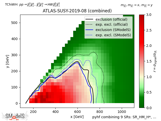
pyhf combining 9 signal regions |
Figure: Comparison of exclusion curves for ATLAS-SUSY-2019-08 using only the best signal region (left), and the combination of all 9 signal regions with pyhf (right).
Combination of different Analyses
Starting with SModelS v2.2, it is possible to combine likelihoods from different analyses, assuming that their signal regions are approximately uncorrelated. As of now, the information of which analyses meet this criterion is not given by SModelS itself, and has to be provided by the user (see option combineAnas).
For these combinations, the combined likelihood \(\mathcal{L}_{C}\) is simply the product of the individual analysis likelihoods, \(\mathcal{L}_{i}\). Furthermore, we assume a common signal strength \(\mu\) for all analyses:
The individual likelihoods can correspond to the best signal region, if the combination of signal regions is turned off, or to the combined signal region likelihood otherwise. For the determination of the maximum likelihood, scipy.optimize.minimize is used with the method BFGS in order to compute \(\hat{\mu}\) and \(\mathcal{L}_{max} = \mathcal{L}_{C}(\hat{\mu})\).
The resulting likelihood and \(r\)-values for the combination are displayed in the output along with the individual results for each analysis.
- 1
The statistical significance of the exclusion statement is difficult to quantify exactly, since the model is being tested by a large number of results simultaneously.
- 2(1,2)
If the root can not be found using the TOMS algorithm, the scipy Brent bracketing algorithm is employed.