Decomposition into Simplified Models
Given an input model, the first task of SModelS is to decompose the full model into a sum of Simplified Models (or elements in SModelS language). Based on the input format, which can be
- a SLHA file or
- a LHE file
(see Basic Input), two distinct (but similar) decomposition methods are applied: the SLHA-based or the LHE-based decomposition.
SLHA-based Decomposition
The SLHA file describing the input model is required to contain the masses of all the BSM states as well as their production cross sections, decay widths and branching ratios. All the above information must follow the guidelines of the SLHA format. In particular, the cross sections also have to be included as SLHA blocks according to the SLHA cross section format.
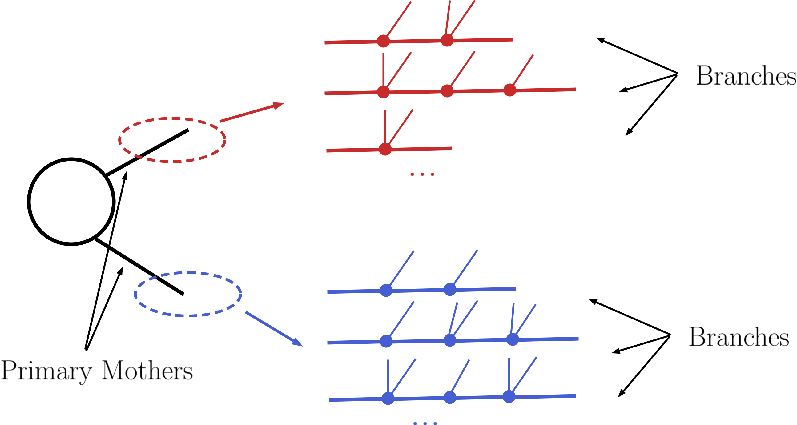
Once the production cross sections are read from the input file, all the cross sections for production of two Z2-odd states are stored and serve as the initial step for the decomposition. (All the other cross sections with a different number of Z2-odd states are ignored.) Starting from these primary mothers, all the possible decays are generated according to the information contained in the DECAY blocks. This procedure is represented in the figure below:
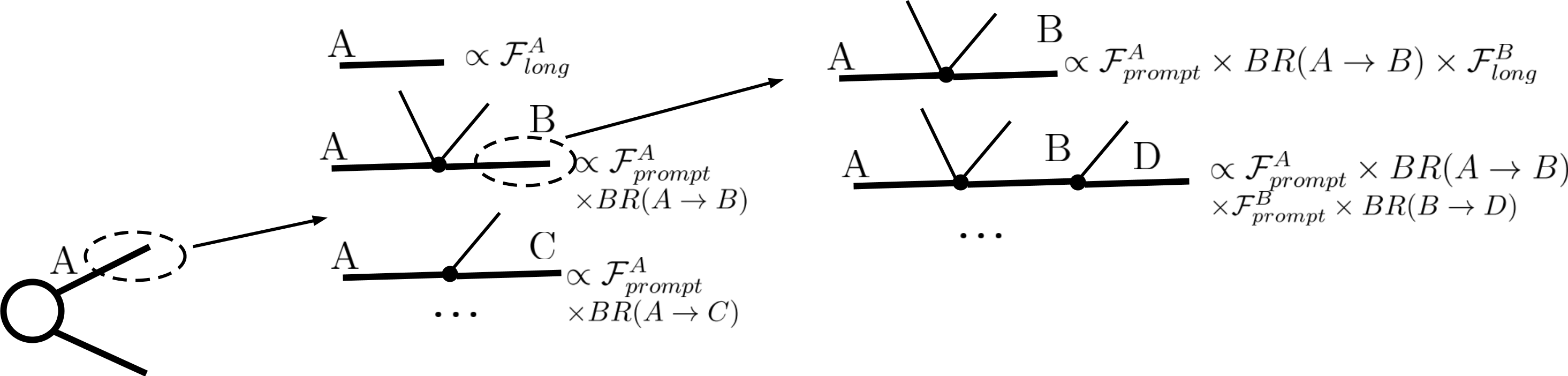
Within SModelS all BSM particles are assumed to either decay promptly or to be stable (in detector scales). To deal with BSM particles with small (non-zero) width SModelS computes the probability for prompt decay (\(\mathcal{F}_{prompt}\)) as well as the probability for the particle to decay outside the detector (\(\mathcal{F}_{long}\)). Note that decays within the detector (displaced decays) are not included in the decomposition. The branching fraction rescaled by \(\mathcal{F}_{long}\) describes the probability of a decay where the daughter BSM state traverses the detector (thus is considered stable), while the branching fraction rescaled by \(\mathcal{F}_{prompt}\) corresponds to a prompt decay which will be followed by the next step in the cascade decay. This reweighting is illustrated in the figure below:
The precise values of \(\mathcal{F}_{prompt}\) and \(\mathcal{F}_{long}\) depend on the relevant detector size (\(L\)), particle mass (\(M\)), boost (\(\beta\)) and width (\(\Gamma\)), thus requiring a Monte Carlo simulation for each input model. Since this is not within the spirit of the simplified model approach, we approximate the prompt and long-lived probabilities by:
where \(L_{outer}\) is the effective size of the detector (which we take to be 10 m for both ATLAS and CMS), \(L_{inner}\) is the effective radius of the inner detector (which we take to be 1 mm for both ATLAS and CMS). Finally, we take the effective time dilation factor to be \(\langle \gamma \beta \rangle = 1.3\) when computing \(\mathcal{F}_{prompt}\) and \(\langle \gamma \beta \rangle = 1.43\) when computing \(\mathcal{F}_{long}\). We point out that the above approximations are irrelevant if \(\Gamma\) is very large (\(\mathcal{F}_{prompt} \simeq 1\) and \(\mathcal{F}_{long} \simeq 0\)) or close to zero (\(\mathcal{F}_{prompt} \simeq 0\) and \(\mathcal{F}_{long} \simeq 1\)). Only elements containing particles which have a considerable fraction of displaced decays will be sensitive to the values chosen above. Furthermore, note that the above procedure discards the fraction of decays which take place within the detector (displaced decays). These are not considered by SModelS, since it can not currently handle displaced decay signatures.
Following the above procedure it is possible to construct all cascade decay possibilities (including the stable case) for a given initial mother particle. Within the SModelS language each of the possible cascade decays corresponds to a branch. In order to finally generate elements, all the branches are combined in pairs according to the production cross sections, as shown below:
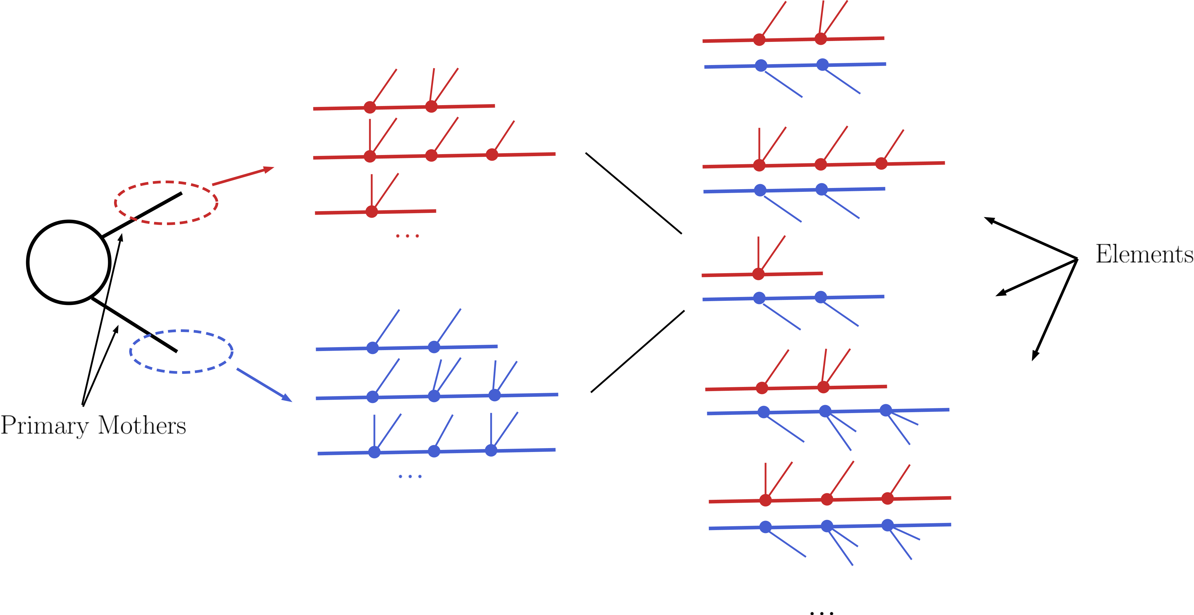
For instance, assume [b1,b2,b3] and [B1,B2] represent all possible branches (or cascade decays) for the primary mothers A and B, respectively. Then, if a production cross section for \(pp \rightarrow A+B\) is given in the input file, the following elements will be generated:
[b1,B1], [b1,B2], [b2,B1], [b2,B2], [b3,B1] and [b3,B2]
Each of the elements generated according to the procedure just described will also store its weight, which equals its production cross section times all the branching ratios appearing in it. In order to avoid a too large number of elements, only those satisfying a minimum weight requirement are kept. Furthermore, the elements are grouped according to their topologies. The final output of the SLHA decomposition is a list of such topologies, where each topology contains a list of the elements generated during the decomposition.
- The SLHA decomposition is implemented by the SLHA decompose method
Minimum Decomposition Weight
Some models may contain a large number of new states and each may have a large number of possible decays. As a result, long cascade decays are possible and the number of elements generated by the decomposition process may become too large, and the computing time too long. For most practical purposes, however, elements with extremely small weights (cross section times BRs times the width rescaling) can be discarded, since they will fall well below the experimental limits. Therefore, during the SLHA decomposition, whenever an element is generated with a weight below some minimum value, this element (and all elements derived from it) is ignored. The minimum weight to be considered is given by the sigcut parameter and is easily adjustable (see slhaDecomposer.decompose).
Note that, when computing the theory predictions, the weight of several elements can be combined together. Hence it is recommended to set the value of sigcut approximately one order of magnitude below the minimum signal cross sections the experimental data can constrain.
LHE-based Decomposition
More general models can be input through an LHE event file containing parton-level events, including the production of the primary mothers and their cascade decays. Each event can then be directly mapped to an element with the element weight corresponding to the event weight. Finally, identical elements can be combined together (adding their weights). The procedure is represented in the example below:
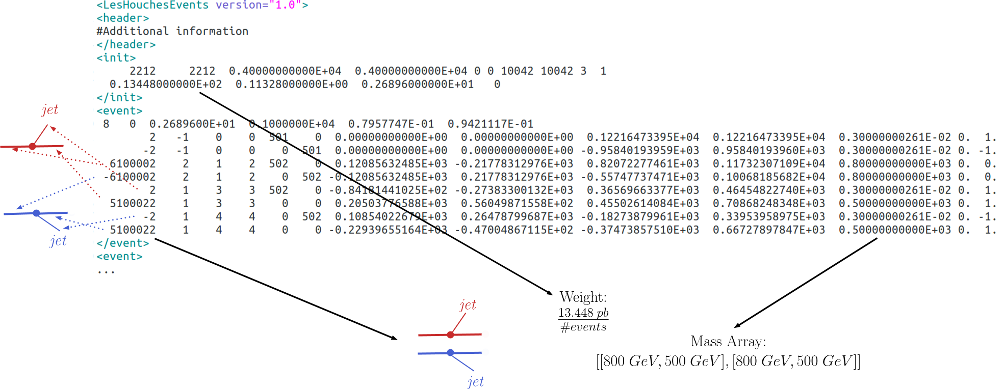
Notice that, for the LHE decomposition, the elements generated are restricted to the events in the input file. Hence, the uncertainties on the elements weights (and which elements are actually generated by the model) are fully dependent on the Monte Carlo statistics used to generate the LHE file. Also, when generating the events it is important to ensure that no mass smearing is applied, so the events always contain the same mass value for a given particle.
Note that since all decays appearing in an LHE event are assumed to be prompt, the LHE-based decomposition should not be used for models with meta-stable BSM particles.
- The LHE decomposition is implemented by the LHE decompose method
Compression of Elements
During the decomposition process it is possible to perform several simplifications on the elements generated. In both the LHE and SLHA-based decompositions, two useful simplifications are possible: Mass Compression and Invisible Compression. The main advantage of performing these compressions is that the simplified element is always shorter (has fewer cascade decay steps), which makes it more likely to be constrained by experimental results. The details behind the compression methods are as follows:
Mass Compression
In case of small mass differences, the decay of an intermediate state to a nearly degenerate one will in most cases produce soft final states, which can not be experimentally detected. Consequently, it is a good approximation to neglect the soft final states and compress the respective decay, as shown below:

After the compression, only the lightest of the two near-degenerate masses are kept in the element, as shown above. The main parameter which controls the compression is minmassgap, which corresponds to the maximum value of \(\epsilon\) in the figure above to which the compression is performed:
Note that the compression is an approximation since the final states, depending on the boost of the parent state, may not always be soft. It is recommended to choose values of minmassgap between 1-10 GeV; the default value is 5 GeV.
- Mass compression is implemented by the massCompress method and can be easily turned on/off by the flag doCompress in the SLHA or LHE decompositions.
Invisible Compression
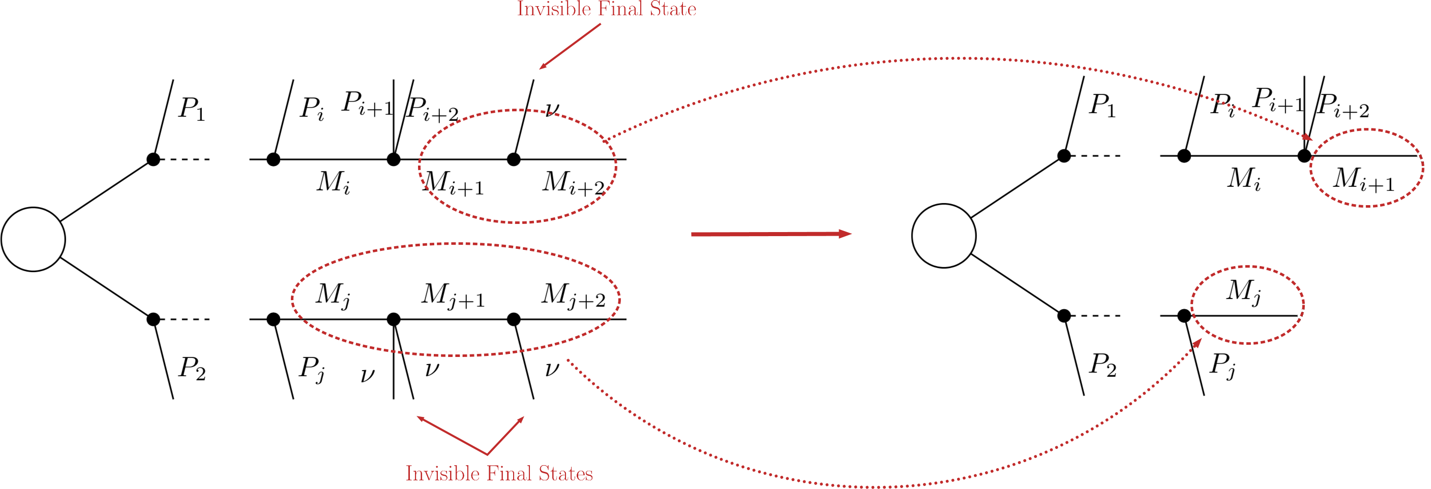
Another type of compression is possible when the final states of the last decay are invisible. The most common example is
as the last step of the decay chain, where \(B\) is an insivible particle leading to a MET signature (see final state class). Since both the neutrino and \(B\) are invisible, for all experimental purposes the effective MET object is \(B + \nu = A\). Hence it is possible to omit the last step in the cascade decay, resulting in a compressed element. Note that this compression can be applied consecutively to several steps of the cascade decay if all of them contain only invisible final states:
- Invisible compression is implemented by the invisibleCompress method and can be easily turned on/off by the flag doInvisible in the SLHA or LHE decompositions.
Element Sorting
In order to improve the code performance, elements created during decomposition and sharing a commong topology are sorted. Sorting allows for an easy ordering of the elements belonging to a topology and faster element comparison. Elements are sorted according to their branches. Branches are compared according to the following properties:
- Number of vertices
- Number of final states in each vertex
- Final state (Z2-even) particles (particles belonging to the same vertex are alphabetically sorted)
- Mass array
- Final state signature
As an example, consider the three elements below:
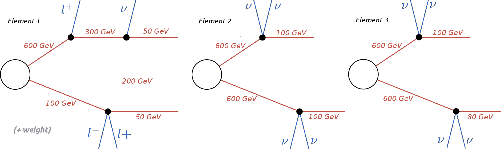
The correct ordering of the above elements is:
Element 3 < Element 2 < Element 1
Element 1 is ‘larger’ than the other two since it has a larger number of vertices. Elements 2 and 3 are identical, except for their masses. Since the mass array of Element 3 is smaller than the one in Element 2, the former is ‘smaller’ than the latter. Finally if all the branch features listed above are identical for both branches, the elements being compared are considered to be equal. Futhermore, the branches belonging to the same element are also sorted. Hence, if an element has two branches:
it implies
- Branch sorting is implemented by the sortBranches method