Database of Experimental Results
SModelS stores all the information about the experimental results in the Database. Below we describe both the directory and object structure of the Database.
Database: Directory Structure
The Database is organized as files in an ordinary (UNIX) directory hierarchy, with a thin Python layer serving as the access to the database. The overall structure of the directory hierarchy and its contents is depicted in the scheme below (click to enlarge):
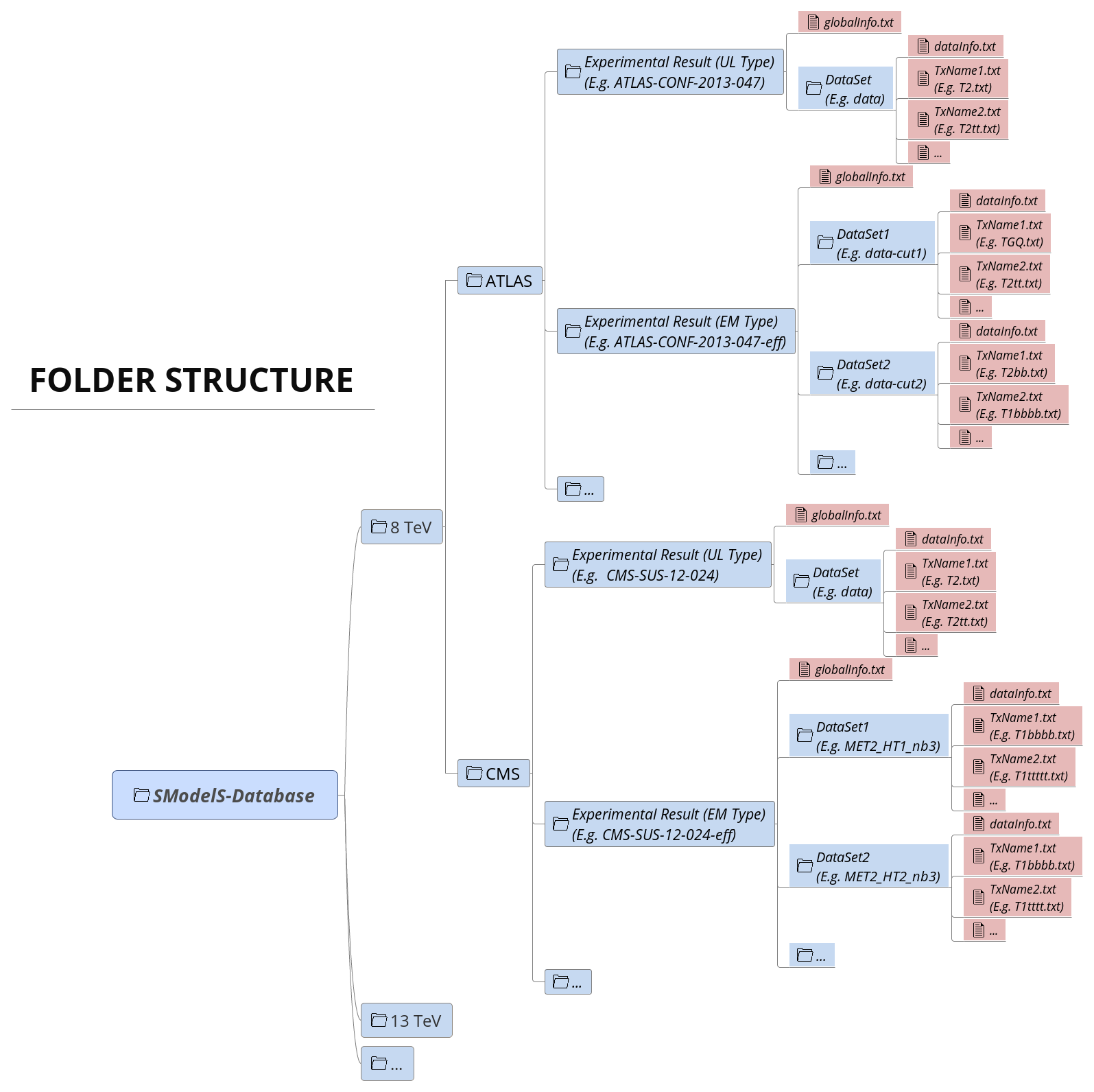
As seen above, the top level of the SModelS database categorizes the analyses by LHC center-of-mass energies, \(\sqrt{s}\):
- 8 TeV
- 13 TeV
Also, the top level directory contains a file called version with the
version string of the database.
The second level splits the results up between the different experiments:
- 8TeV/CMS/
- 8TeV/ATLAS/
The third level of the directory hierarchy encodes the Experimental Results:
- 8TeV/CMS/CMS-SUS-12-024
- 8TeV/ATLAS/ATLAS-CONF-2013-047
- …
- The Database folder is described by the Database Class
Experimental Result Folder
Each Experimental Result folder contains:
- a folder for each DataSet (e.g.
data) - a
globalInfo.txtfile
The globalInfo.txt file contains the meta information about the Experimental Result.
It defines the center-of-mass energy \(\sqrt{s}\), the integrated luminosity, the id
used to identify the result and additional information about the source of the
data. Here is the content of CMS-SUS-12-024/globalInfo.txt as an example:
sqrts: 8.0*TeV
lumi: 19.4/fb
id: CMS-SUS-12-024
prettyName: \slash{E}_{T}+b
url: https://twiki.cern.ch/twiki/bin/view/CMSPublic/PhysicsResultsSUS12024
arxiv: http://arxiv.org/abs/1305.2390
publication: http://www.sciencedirect.com/science/article/pii/S0370269313005339
contact: Keith Ulmer <keith.ulmer@cern.ch>, Josh Thompson <joshua.thompson@cern.ch>, Alessandro Gaz <alessandro.gaz@cern.ch>
private: False
implementedBy: Wolfgang Waltenberger
lastUpdate: 2015/5/11
- Experimental Result folder is described by the ExpResult Class
- globalInfo files are descrived by the Info Class
Data Set Folder
Each DataSet folder (e.g. data) contains:
- the Upper Limit maps for UL-type results or Efficiency maps for EM-type results (
TxName.txtfiles) - a
dataInfo.txtfile containing meta information about the DataSet - Data Set folders are described by the DataSet Class
- TxName files are described by the TxName Class
- dataInfo files are described by the Info Class
Data Set Folder: Upper Limit Type
Since UL-type results have a single dataset (see DataSets), the info file only holds some trivial information, such as the type of Experimental Result (UL) and the dataset id (None for UL-type results). Here is the content of CMS-SUS-12-024/data/dataInfo.txt as an example:
dataType: upperLimit
dataId: None
For UL-type results, each TxName.txt file contains the UL map for a given simplified model
(element or sum of elements) as well as some meta information,
including the corresponding constraint and conditions. The
first few lines of CMS-SUS-12-024/data/T1tttt.txt read:
txName: T1tttt
constraint: [[['t','t']],[['t','t']]]
condition: None
conditionDescription: None
figureUrl: https://twiki.cern.ch/twiki/pub/CMSPublic/PhysicsResultsSUS12024/T1tttt_exclusions_corrected.pdf
source: CMS
validated: True
axes: [[x, y], [x, y]]
If the finalState property is not provided, the simplified model is assumed to
contain neutral BSM final states in each branch, leading to a MET signature.
However, if this is not the case, the non-MET final states must be explicitly listed
in the TxName.txt file (see final state classes for more details).
An example from the CMS-EXO-12-026/data/THSCPM1b.txt file is shown below:
txName: THSCPM1b
constraint: [[],[]]
source: CMS
axes: [[x], [x]]
finalState: ['HSCP', 'HSCP']
The second block of data in the TxName.txt file contains the upper limits as a function of the BSM masses:
upperLimits: [[[[4.0000E+02*GeV,0.0000E+00*GeV],[4.0000E+02*GeV,0.0000E+00*GeV]],1.8158E+00*pb],
[[[4.0000E+02*GeV,2.5000E+01*GeV],[4.0000E+02*GeV,2.5000E+01*GeV]],1.8065E+00*pb],
[[[4.0000E+02*GeV,5.0000E+01*GeV],[4.0000E+02*GeV,5.0000E+01*GeV]],2.1393E+00*pb],
[[[4.0000E+02*GeV,7.5000E+01*GeV],[4.0000E+02*GeV,7.5000E+01*GeV]],2.4721E+00*pb],
[[[4.0000E+02*GeV,1.0000E+02*GeV],[4.0000E+02*GeV,1.0000E+02*GeV]],2.9297E+00*pb],
[[[4.0000E+02*GeV,1.2500E+02*GeV],[4.0000E+02*GeV,1.2500E+02*GeV]],3.3874E+00*pb],
[[[4.0000E+02*GeV,1.5000E+02*GeV],[4.0000E+02*GeV,1.5000E+02*GeV]],3.4746E+00*pb],
[[[4.0000E+02*GeV,1.7500E+02*GeV],[4.0000E+02*GeV,1.7500E+02*GeV]],3.5618E+00*pb],
[[[4.2500E+02*GeV,0.0000E+00*GeV],[4.2500E+02*GeV,0.0000E+00*GeV]],1.3188E+00*pb],
[[[4.2500E+02*GeV,2.5000E+01*GeV],[4.2500E+02*GeV,2.5000E+01*GeV]],1.3481E+00*pb],
[[[4.2500E+02*GeV,5.0000E+01*GeV],[4.2500E+02*GeV,5.0000E+01*GeV]],1.7300E+00*pb],
As we can see, the UL map is given as a Python array with the structure: \([[\mbox{masses},\mbox{upper limit}], [\mbox{masses},\mbox{upper limit}],...]\).
Data Set Folder: Efficiency Map Type
For EM-type results the dataInfo.txt contains relevant information, such as an id to
identify the DataSet (signal region), the number of observed and expected
background events for the corresponding signal region and the respective signal
upper limits. Here is the content of
CMS-SUS-13-012-eff/3NJet6_1000HT1250_200MHT300/dataInfo.txt as an example:
dataType: efficiencyMap
dataId: 3NJet6_1000HT1250_200MHT300
observedN: 335
expectedBG: 305
bgError: 41
upperLimit: 5.681*fb
expectedUpperLimit: 4.585*fb
For EM-type results, each TxName.txt file contains the efficiency map for a given
simplified model (element or sum of elements) as well as some meta
information.
Here is the first few lines of CMS-SUS-13-012-eff/3NJet6_1000HT1250_200MHT300/T2.txt:
txName: T2
conditionDescription: None
condition: None
constraint: [[['jet']],[['jet']]]
figureUrl: https://twiki.cern.ch/twiki/pub/CMSPublic/PhysicsResultsSUS13012/Fig_7a.pdf
validated: True
axes: 2*Eq(mother,x)_Eq(lsp,y)
publishedData: False
As seen above, the first block of data in the T2.txt file contains
information about the element (\([[[\mbox{jet}]],[[\mbox{jet}]]]\))
in bracket notation for which the
efficiencies refers to as well as reference to the original data source and
some additional information.
As in the Upper Limit case, the simplified
model is assumed to contain neutral BSM final states (MET signature).
For non-MET final states the finalState field must list
the final state signatures.
The second block of data contains the efficiencies as a function of the BSM masses:
efficiencyMap: [[[[312.5*GeV, 12.5*GeV], [312.5*GeV, 12.5*GeV]], 0.00109],
[[[312.5*GeV, 62.5*GeV], [312.5*GeV, 62.5*GeV]], 0.00118],
[[[312.5*GeV, 112.5*GeV], [312.5*GeV, 112.5*GeV]], 0.00073],
[[[312.5*GeV, 162.5*GeV], [312.5*GeV, 162.5*GeV]], 0.00044],
	...
As we can see the efficiency map is given as a Python array with the structure: \([[\mbox{masses},\mbox{efficiency}], [\mbox{masses},\mbox{efficiency}],...]\).
Inclusive Simplified Models
If the analysis signal efficiencies are insensitive to some of the simplified model final states, it might be convenient to define inclusive simplified models. A typical case are some of the heavy stable charged particle searches, which only rely on the presence of a non-relativistic charged particle, which leads to an anomalous charged track signature. In this case the signal efficiencies are highly insensitive to the remaining event activity and the corresponding simplified models can be very inclusive. In order to handle this inclusive cases in the database we allow for wildcards when specifying the constraints. For instance, the constraint for the CMS-EXO-13-006 eff/c000/THSCPM3.txt reads:
txName: THSCPM3
constraint: [[['*']],[['*']]]
and represents the (inclusive) simplified model:
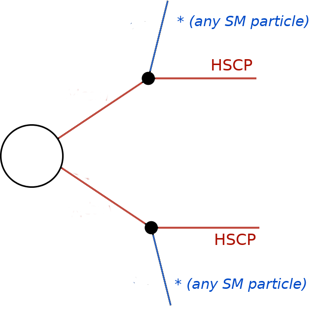
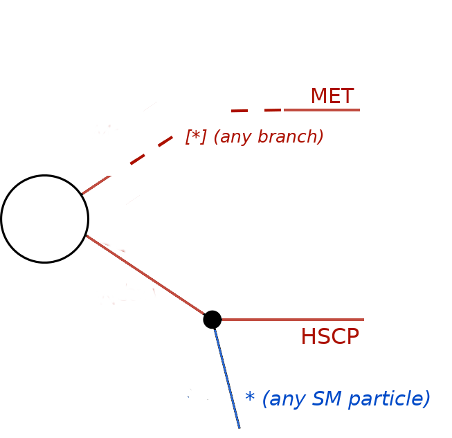
Note that although the final state represented by “*” is any Z2-even final states, it must still correspond to a single particle, since the topology specifies a 2-body decay for the initially produced BSM particle. Finally, it might be useful to define even more inclusive simplified models, such as the one in CMS-EXO-13-006 eff/c000/THSCPM4.txt:
txName: THSCPM4
constraint: [[*],[['*']]]
finalState: ['MET', 'HSCP']
In the above case the simplified model corresponds to an HSCP being initially produced in association with any BSM particle which leads to a MET signature. Notice that the notation “[*]” corresponds to any `branch, while [“*”] means any particle:
In such cases the mass array for the arbitrary branch must also be specified as using wildcards:
efficiencyMap: [[['*',[5.5000E+01*GeV,5.0000E+01*GeV]],5.27e-06],
[['*',[1.5500E+02*GeV,5.0000E+01*GeV]],1.28e-07],
[['*',[1.5500E+02*GeV,1.0000E+02*GeV]],0.13],
Database: Object Structure
The Database folder structure is mapped to Python objects in SModelS. The mapping is almost one-to-one, except for a few exceptions. Below we show the overall object structure as well as the folders/files the objects represent (click to enlarge):
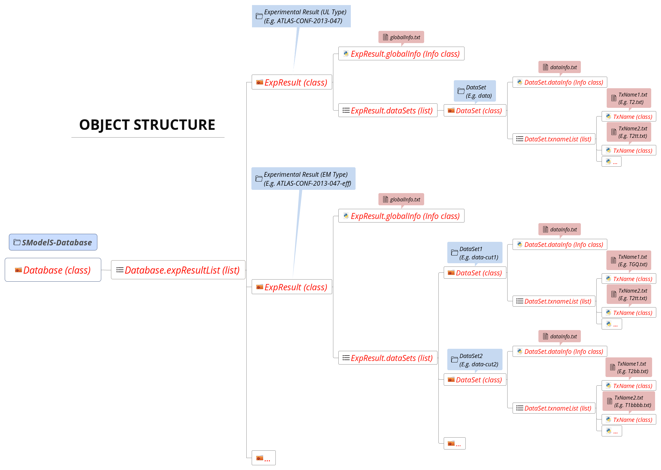
The type of Python object (Python class, Python list,…) is shown in brackets. For convenience, below we explicitly list the main database folders/files and the Python objects they are mapped to:
- Database folder \(\rightarrow\) Database Class
- Experimental Result folder \(\rightarrow\) ExpResult Class
- DataSet folder \(\rightarrow\) DataSet Class
globalInfo.txtfile \(\rightarrow\) Info ClassdataInfo.txtfile \(\rightarrow\) Info ClassTxname.txtfile \(\rightarrow\) TxName Class
Database: Binary (Pickle) Format
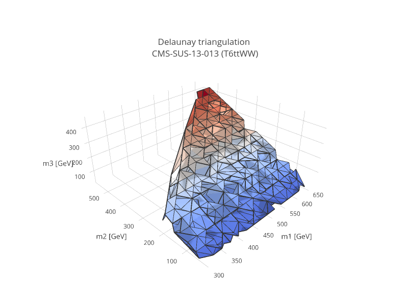
At the first time of instantiating the Database class, the text files in <database-path>. are loaded and parsed, and the corresponding data objects are built. The efficiency and upper limit maps themselves are subjected to standard preprocessing steps such as a principal component analysis and Delaunay triangulation (see Figure below). The simplices defined during triangulation are then used for linearly interpolating the data grid, thus allowing SModelS to compute efficiencies or upper limits for arbitrary mass values (as long as they fall inside the data grid). This procedure provides an efficient and numerically robust way of dealing with generic data grids, including arbitrary parametrizations of the mass parameter space, irregular data grids and asymmetric branches.
For the sake of efficiency, the entire database – including the Delaunay triangulation – is then serialized into a pickle file (<database-path>/database.pcl), which will be read directly the next time the database is loaded. If any changes in the database folder structure are detected, the python or the SModelS version has changed, SModelS will automatically re-build the pickle file. This action may take a few minutes, but it is again performed only once. If desired, the pickling process can be skipped using the option force_load = `txt’ in the constructor of Database .
- The pickle file is created by the createBinaryFile method