Theory Predictions
The decomposition of the input model as a sum of elements (simplified models) is the first step for confronting the model with the experimental limits. The next step consists of computing the relevant signal cross sections (or theory predictions) for comparison with the experimental limits. Below we describe the procedure for the computation of the theory predictions after the model has been decomposed.
Computing Theory Predictions
As discussed in Database Definitions, the SModelS database allows for two types of experimental constraints: Upper Limit constraints (see UL-type results) and Efficiency Map constraints (see EM-type results). Each of them requires different theoretical predictions to be compared against experimental data.
UL-type results constrains the weight (\(\sigma \times BR\)) of one element or sum of elements. Therefore SModelS must compute the theoretical value of \(\sigma \times BR\) summing only over the elements appearing in the respective constraint. This is done by assigning an efficiency equal to 1 (0) to each element, if the element appears (does not appear) in the constraint. Then the final theoretical prediction is the sum over all elements with a non-zero value of \(\sum \sigma \times BR \times \epsilon\). This value can then be compared with the respective 95% C.L. upper limit extracted from the UL map (see UL-type results).
On the other hand, EM-type results constrain the total signal (\(\sum \sigma \times BR \times \epsilon\)) in a given signal region (DataSet). Consequently, in this case SModelS must compute \(\sigma \times BR \times \epsilon\) for each element, using the efficiency maps for the corresponding DataSet. The final theoretical prediction is the sum over all elements with a non-zero value of \(\sigma \times BR \times \epsilon\). This value can then be compared with the signal upper limit for the respective signal region (data set).
For experimental results for which the covariance matrix is provided, it is possible to combine all the signal regions (see Combination of Signal Regions). In this case the final theory prediction corresponds to the sum of \(\sigma \times BR \times \epsilon\) over all signal regions (and all elements) and the upper limit is computed for this sum.
Although the details of the theoretical prediction computation differ depending on the type of Experimental Result (UL-type results or EM-type results), the overall procedure is common for both types of results. Below we schematically show the main steps of the theory prediction calculation:
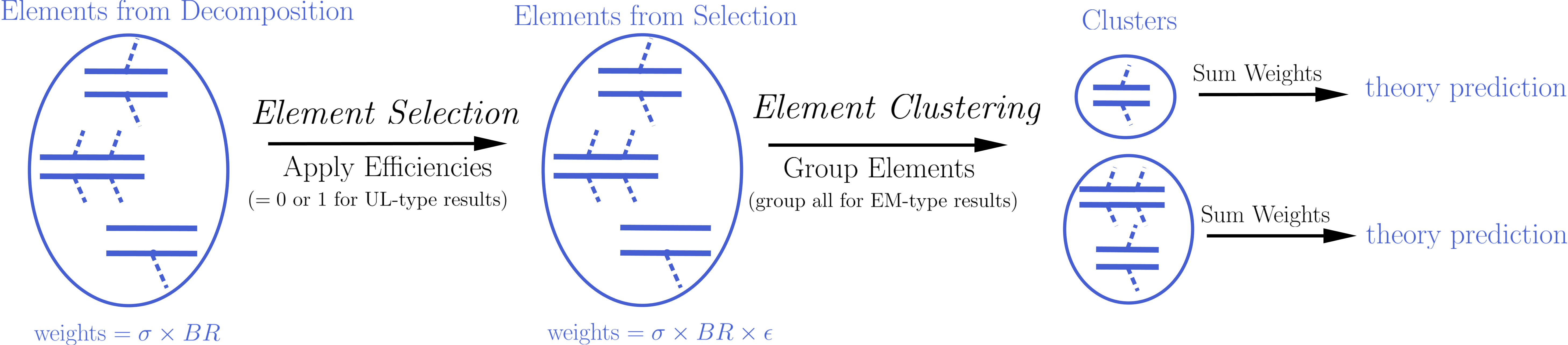
As shown above the procedure can always be divided in two main steps: Element Selection and Element Clustering. Once the elements have been selected and clustered, the theory prediction for each DataSet is given by the sum of all the element weights (\(\sigma \times BR \times \epsilon\)) belonging to the same cluster:
Below we describe in detail the element selection and element clustering methods for computing the theory predictions for each type of Experimental Result separately.
- Theory predictions are computed using the theoryPredictionsFor method
Theory Predictions for Upper Limit Results
Computation of the signal cross sections for a given UL-type result takes place in two steps. First selection of the elements generated by the model decomposition and then clustering of the selected elements according to their properties. These two steps are described below.
Element Selection
An UL-type result holds upper limits for the cross sections of an element or sum of elements. Consequently, the first step for computing the theory predictions for the corresponding experimental result is to select the elements that appear in the UL result constraint. This is conveniently done attributing to each element an efficiency equal to 1 (0) if the element appears (does not appear) in the constraint. After all the elements weights (\(\sigma \times BR\)) have been rescaled by these ‘’trivial’’ efficiencies, only the ones with non-zero weights are relevant for the signal cross section. The element selection is then trivially achieved by selecting all the elements with non-zero weights.
The procedure described above is illustrated graphically in the figure below for the simple example where the constraint is \([[[e^+]],[[e^-]]]\,+\,[[[\mu^+]],[[\mu^-]]]\).
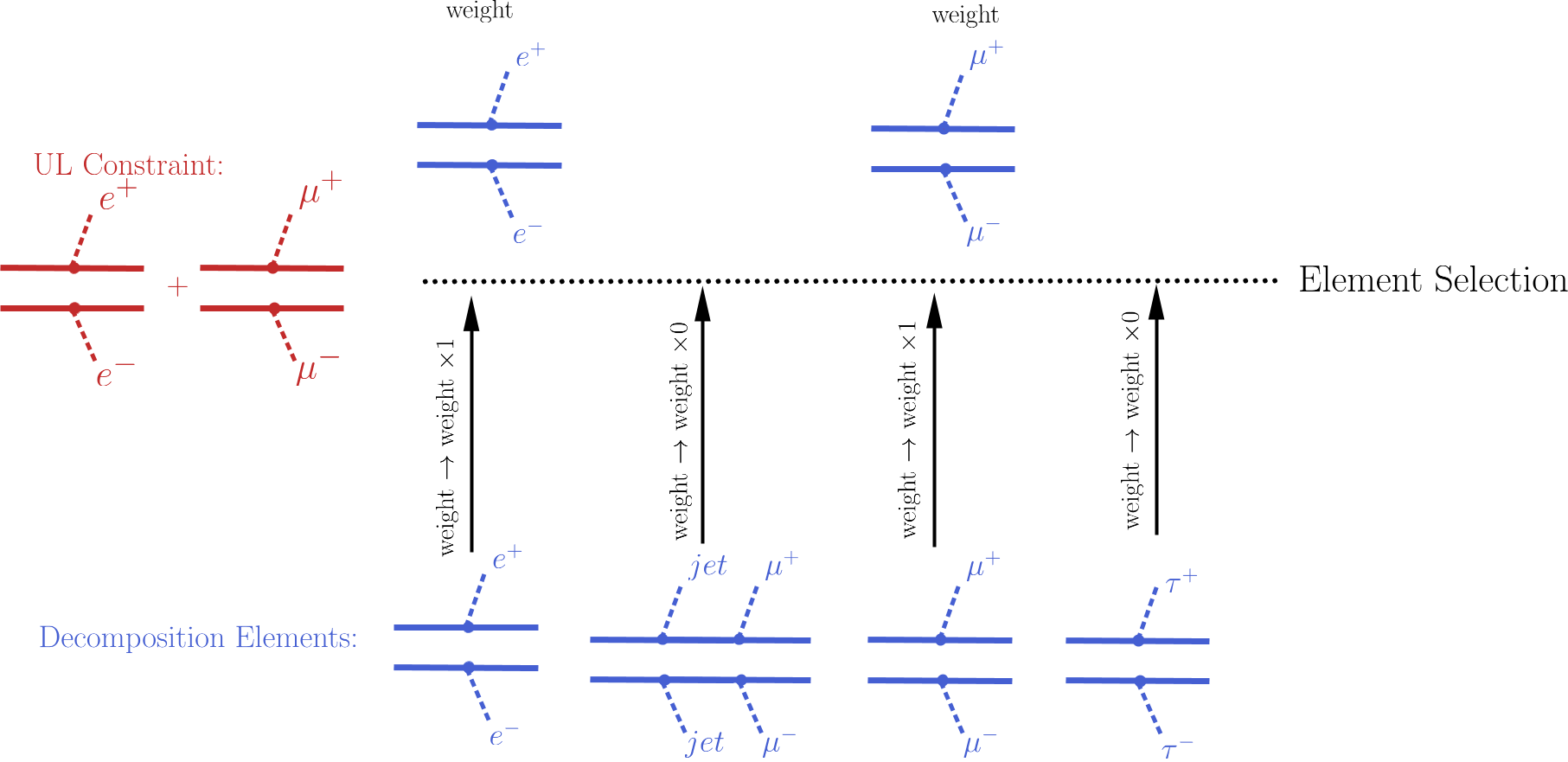
- The element selection is implemented by the getElementsFrom method
Element Clustering
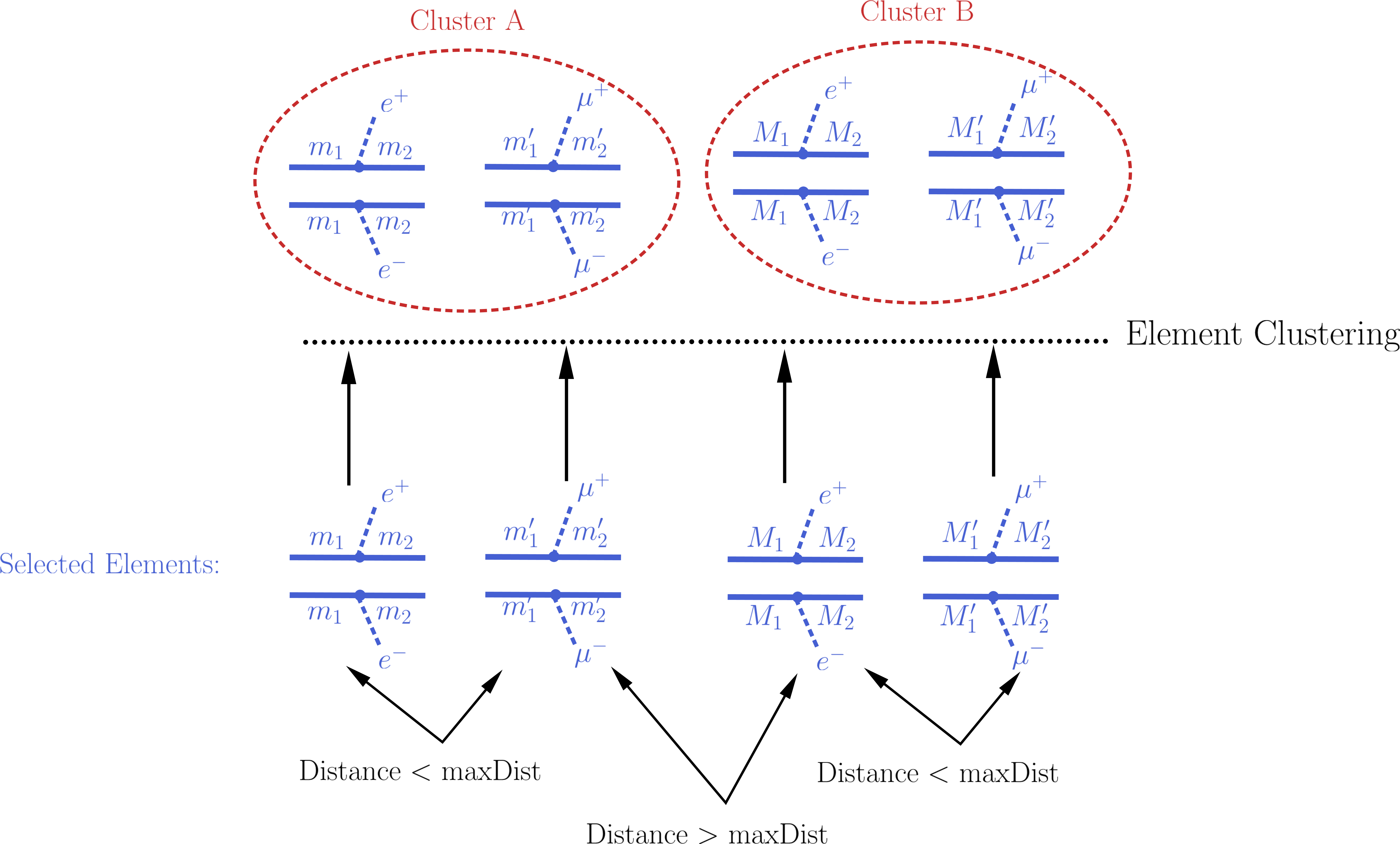
Naively one would expect that after all the elements appearing in the constraint have been selected, it is trivial to compute the theory prediction: one must simply sum up the weights (\(\sigma \times BR\)) of all the selected elements. However, the selected elements usually differ in their masses and/or widths[1] and the experimental limit (see Upper Limit constraint) assumes that all the elements appearing in the constraint have the same efficiency, which typically implies that the distinct elements have the same mass arrays and widths. As a result, the selected elements must be grouped into clusters of equal masses and widths. When grouping the elements, however, one must allow for small differences, since the experimental efficiencies should not be strongly sensitive to tiny changes in mass or width values. For instance, assume two elements contain identical mass arrays, except for the parent masses which differ by 1 MeV. In this case it is obvious that for all experimental purposes the two elements have the same mass and should contribute to the same theory prediction (e.g. their weights should be added when computing the signal cross section). Unfortunately there is no way to unambiguously define ‘’similar efficiencies’’ or ‘’similar masses and widths’’ and the definition should depend on the Experimental Result. In the simplest case where the upper limit result corresponds to a single signal region (which is not always the case), one could assume that each element efficiency is inversely proportional to its upper limit. Hence the distance between two elements can be defined as the relative difference between their upper limits, as described in element distance. Then, if the distance between two selected elements is smaller than a maximum value (defined by maxDist), they are gouped in the same cluster and their cross-sections will be combined, as illustrated by the example below:
Notice that the above definition of distance quantifies the experimental analysis sensitivity to changes in the element properties (masses and widths), which should correspond to changes in the upper limit value for the element. However, most Experimental Results combine distinct signal regions or use a more complex analysis in order to derive upper limits. In such cases, two elements can have (by chance) the same upper limit value, but still have very distinct efficiencies and should not be considered similar and combined. In order to deal with such cases an additional requirement is imposed when clustering two elements: the distance between both elements to the average element must also be smaller than maxDist . The average element of a list of elements corresponds to the element with the same common topology and final states, but with the mass array and widths replaced by the average mass and width over all the elements in the list. If this average element has an upper limit similar to all the elements in the list, we assume that all the elements have similar efficiencies and can be considered as similar to the given Experimental Result.
Once all the elements have been clustered, their weights can finally be added together and compared against the experimental upper limit.
- The clustering of elements is implemented by the clusterElements method.
Distance Between Elements
As mentioned above, in order to cluster the elements it is necessary to determine whether two elements are similar for a given Experimental Result. This usually means that both elements have similar efficiencies for the Experimental Result. Since an absolute definition of ‘’similar elements’’ is not possible and the sensitivity to changes in the mass or width of a given element depends on the experimental result, SModelS uses an ‘’upper limit map-dependent’’ definition. Each element is mapped to its corresponding upper limit for a given Experimental Result and the distance between two elements is simply given by the relative distance between the upper limits:
Theory Predictions for Efficiency Map Results
In order to compute the signal cross sections for a given EM-type result, so it can be compared to the signal region limits, it is first necessary to apply the efficiencies (see EM-type result) to all the elements generated by the model decomposition. Notice that typically a single EM-type result contains several signal regions (DataSets) and there will be a set of efficiencies (or efficiency maps) for each data set. As a result, several theory predictions (one for each data set) will be computed. This procedure is similar (in nature) to the Element Selection applied in the case of a UL-type result, except that now it must be repeated for several data sets (signal regions).
After the element’s weights have being rescaled by the corresponding efficiencies for the given data set (signal region), all of them can be grouped together in a single cluster, which will provide a single theory prediction (signal cross section) for each DataSet. Hence the element clustering discussed below is completely trivial. On the other hand the element selection is slightly more involved than in the UL-type result case and will be discussed in more detail.
Element Selection
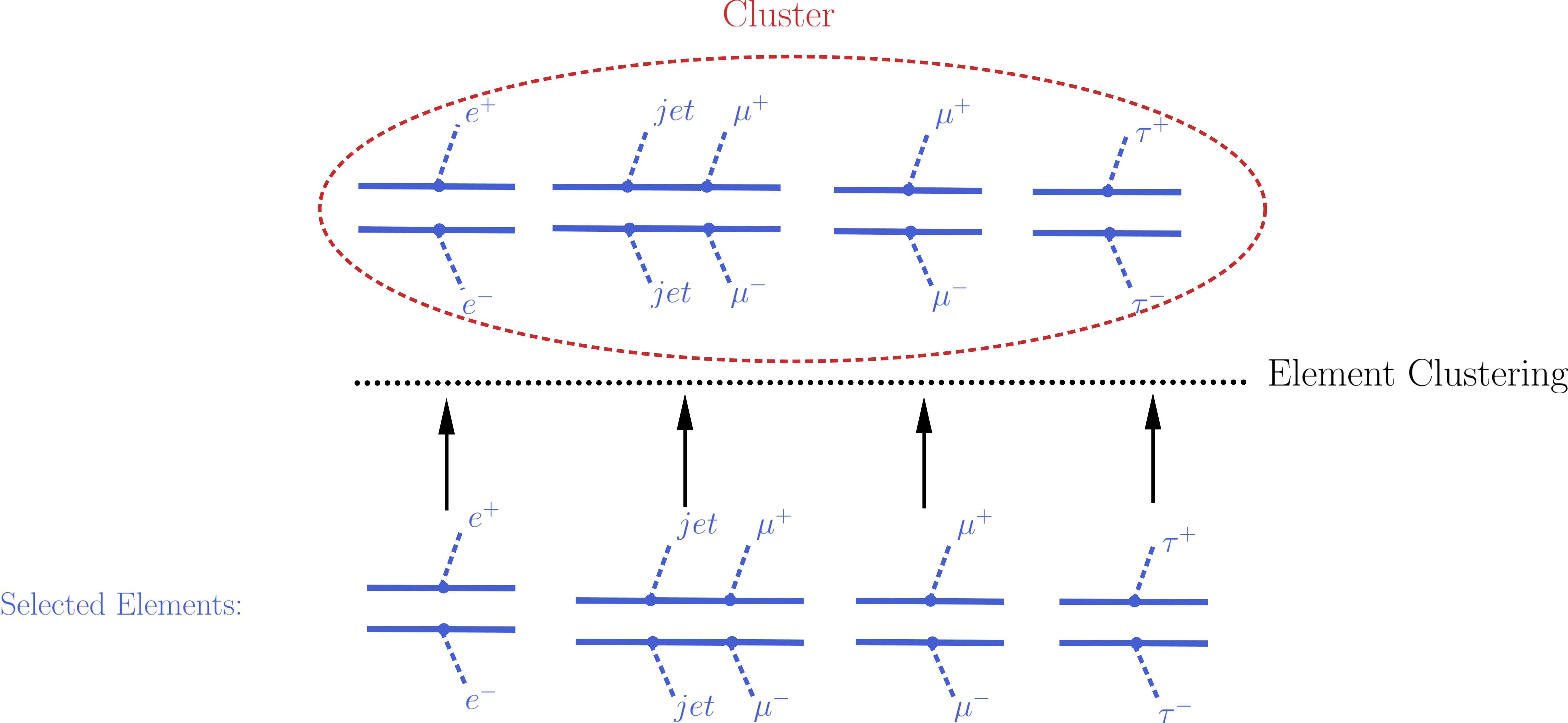
The element selection for the case of an EM-type result consists of rescaling all the elements weights by their efficiencies, according to the efficiency map of the corresponding DataSet. The efficiency for a given DataSet depends both on the element topology and its particle content. In practice the efficiencies for most of the elements will be extremely small (or zero), hence only a subset effectively contributes after the element selection[2]. In the figure below we illustrate the element selection for the case of an EM-type result/DataSet:
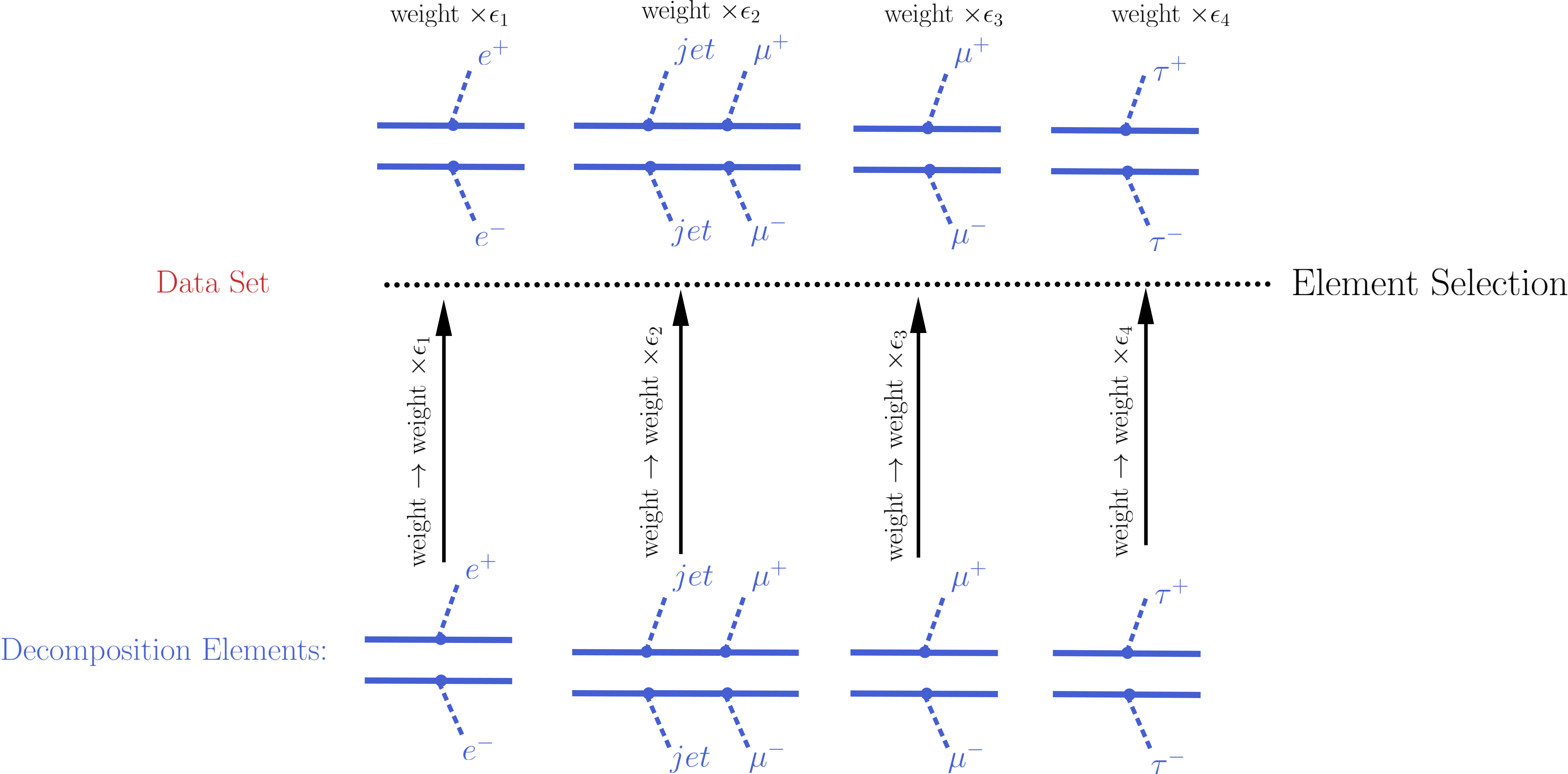
If, for instance, the analysis being considered vetoes \(jets\) and \(\tau\)’s in the final state, we will have \(\epsilon_2,\, \epsilon_4 \simeq 0\) for the example in the figure above. Also, if the experimental result applies only to prompt decays and the element contains intermediate meta-stable BSM particles, its efficiency will be very small (although not necessarily zero).
- The element selection is implemented by the getElementsFrom method
Element Clustering
After the efficiencies have been applied to the element’s weights, all the elements can be combined together when computing the theory prediction for the given DataSet (signal region). Since a given signal region correspond to the same signal upper limit for any element, the distance between any two elements for an EM-type result is always zero and the clustering procedure described above will trivially group together all the selected elements into a single cluster:
- The clustering of elements is implemented by the clusterElements method.
| [1] | When refering to an element mass or width, we mean all the masses and widths of the Z2-odd particles appearing in the element. Two elements are considered to have identical masses and widths if their mass arrays and width arrays are identical. |
| [2] | The number of elements passing the selection also depends on the availability of efficiency maps for the elements generated by the decomposition. Whenever there are no efficiencies available for an element, the efficiency is taken to be zero. |